
Are you struggling with messy, inconsistent data in your database? Do duplicate entries and anomalies slow down your system?
Decomposition in DBMS is your solution.
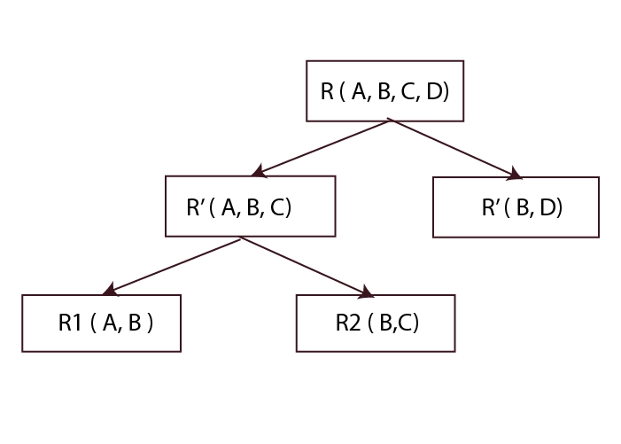
In DBMS, decomposition can be defined as an approach of subdividing a large table into even smaller ones so as to solve complex and large problems. This practice works towards the improvement of quality, reduction of time and effort, as well as eradication of multiple entries of similar data.
In this blog, we will look at what decomposition in DBMS is, why it matters, different types, properties, and more advanced concepts in decomposition and look at the strengths and weaknesses as well.
Importance of Decomposition in DBMS
To effectively manage the cleanliness of the database, decomposition plays an important role. The large tables can be divided into smaller ones, which will allow you to avoid any discrepancies in the data.
Here’s why decomposition matters:
- Improves Data Integrity: Ensures that all data remains accurate and consistent.
- Optimises Storage: Reduces redundancy and saves storage space.
- Enhances Performance: Makes database operations faster and more efficient.
Imagine managing a library. You don’t have one enormous list of all books but rather have subdivisions based on the genre: fiction, non-fiction, etc. This makes it easy for youths to locate and organise books. This makes it easier to find and manage books. Similarly, decomposition organises data in a database.
Also Read: Database Languages in DBMS

POSTGRADUATE PROGRAM IN
Multi Cloud Architecture & DevOps
Master cloud architecture, DevOps practices, and automation to build scalable, resilient systems.
Different Types of Decomposition in DBMS
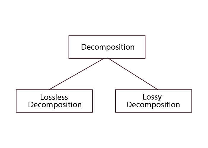
Understanding the types of decomposition is key to applying the right one for your needs. We can categorise decomposition into two types:
- Lossless Decomposition
- Lossy Decomposition
Let’s understand them one by one.
Lossless Decomposition: Ensuring No Data Loss
Lossless decomposition means splitting a table without losing any data. When we join the decomposed tables, we get back to the original table.
This is like cutting a cake into slices and then putting it back together perfectly.
Example
Consider a table StudentCourse:
| StudentID | StudentName | CourseID | CourseName |
| 1 | Divya | 101 | Math |
| 2 | Rahul | 102 | Science |
We decompose it into:
1. Student Table:
| StudentID | StudentName | CourseID |
| 1 | Divya | 101 |
| 2 | Rahul | 102 |
2. Course Table:
| CourseID | CourseName |
| 101 | Math |
| 102 | Science |
By joining these on CourseID, we get the original StudentCourse table back.
Here’s how to do it in Python:
# Example to demonstrate lossless decomposition

# Input data

students = [

{"StudentID": 1, "StudentName": "Divya", "CourseID": 101},

{"StudentID": 2, "StudentName": "Rahul", "CourseID": 102}

]

courses = [

{"CourseID": 101, "CourseName": "Math"},

{"CourseID": 102, "CourseName": "Science"}

]

# Display original data

print("Original Student Data:")

for student in students:

print(student)

print("\nOriginal Course Data:")

for course in courses:

print(course)

# Join operation

result = []

for student in students:

for course in courses:

if student["CourseID"] == course["CourseID"]:

result.append({**student, "CourseName": course["CourseName"]})

# Display joined data

print("\nJoined Data (Lossless):")

for row in result:

print(row)
Output:
Original Student Data:

{'StudentID': 1, 'StudentName': 'Divya', 'CourseID': 101}

{'StudentID': 2, 'StudentName': 'Rahul', 'CourseID': 102}


Original Course Data:

{'CourseID': 101, 'CourseName': 'Math'}

{'CourseID': 102, 'CourseName': 'Science'}


Joined Data (Lossless):

{'StudentID': 1, 'StudentName': 'Divya', 'CourseID': 101, 'CourseName': 'Math'}

{'StudentID': 2, 'StudentName': 'Rahul', 'CourseID': 102, 'CourseName': 'Science'}
Lossy Decomposition: Potential for Data Loss
Lossy decomposition might result in losing some data when we split and then rejoin tables. This is like cutting a cake and losing some crumbs.
Example
Consider a table EmployeeProject:
| EmpID | EmpName | ProjectID | Hours |
| 1 | Amit | 201 | 20 |
| 2 | Anamika | 202 | 30 |
We decompose it into:
1. Employee Table:
| EmpID | EmpName |
| 1 | Amit |
| 2 | Anamika |
2. Project Table:
| ProjectID | Hours |
| 201 | 20 |
| 202 | 30 |
Rejoining these might not accurately recreate the original EmployeeProject table.
Here’s how a lossy decomposition might look in Python:
# Example to demonstrate lossy decomposition

# Input data

employees = [

{"EmpID": 1, "EmpName": "Amit"},

{"EmpID": 2, "EmpName": "Anamika"}

]

projects = [

{"ProjectID": 201, "Hours": 20},

{"ProjectID": 202, "Hours": 30}

]

# Display original data

print("Original Employee Data:")

for employee in employees:

print(employee)

print("\nOriginal Project Data:")

for project in projects:

print(project)

# Join operation (illustrative, showing the potential loss)

result = []

for employee in employees:

for project in projects:

result.append({**employee, **project})

# Display joined data

print("\nJoined Data (Lossy):")

for row in result:

print(row)
Output:
Original Employee Data:

{'EmpID': 1, 'EmpName': 'Amit'}

{'EmpID': 2, 'EmpName': 'Anamika'}


Original Project Data:

{'ProjectID': 201, 'Hours': 20}

{'ProjectID': 202, 'Hours': 30}


Joined Data (Lossy):

{'EmpID': 1, 'EmpName': 'Amit', 'ProjectID': 201, 'Hours': 20}

{'EmpID': 1, 'EmpName': 'Amit', 'ProjectID': 202, 'Hours': 30}

{'EmpID': 2, 'EmpName': 'Anamika', 'ProjectID': 201, 'Hours': 20}

{'EmpID': 2, 'EmpName': 'Anamika', 'ProjectID': 202, 'Hours': 30}
Here, the original relationships between employees and projects are lost, leading to incorrect data.
Key Properties of Decomposition in DBMS
When decomposing tables, keeping these properties in mind ensures success.
Ensuring a Lossless Join in Decomposition
A lossless join is critical. It means that when we join decomposed tables, we should get back to the original table exactly as it was. Here’s how we can ensure a lossless join:
- Union of Attributes: The combined attributes of the decomposed tables must cover all attributes of the original table.
- Common Attribute: There should be at least one common attribute between the decomposed tables, which acts as a superkey.
Maintaining Dependency Preservation During Decomposition
Dependency preservation ensures that all functional dependencies are maintained in the decomposed tables. This is important for maintaining the logical relationships between data.
Reducing Data Redundancy Through Decomposition
Reducing redundancy means eliminating duplicate data entries. This makes the database more efficient and easier to manage.
Enhancing Database Efficiency
By decomposing tables, we can improve database performance. Smaller, well-structured tables make queries and updates faster and more efficient.
Maintaining Data Integrity and Consistency
Decomposition ensures that data remains accurate and consistent. By breaking down tables, we can manage data anomalies better and ensure consistency across the database.
Exploring Lossless Decomposition with Unique Examples
Lossless decomposition ensures that no data is lost when splitting a table. It’s like cutting a cake and being able to piece it back together perfectly. But how do we ensure this?
Criteria for a Lossless Join Decomposition
For a decomposition to be lossless, it must meet these criteria:
- Cover All Attributes: The decomposed tables must include all attributes of the original table.
- Common Superkey: There must be a common attribute that acts as a superkey in one or both tables.
These criteria ensure that we can perfectly recreate the original table by joining the decomposed tables.
Practical Example of a Lossless Decomposition
Imagine a table StudentCourse with columns: StudentID, StudentName, CourseID, and CourseName. Here’s what the table looks like:
| StudentID | StudentName | CourseID | CourseName |
| 1 | Neha | 101 | Math |
| 2 | Rohan | 102 | Science |
We can decompose it into two tables:
1. Student Table:
| StudentID | StudentName | CourseID |
| 1 | Neha | 101 |
| 2 | Rohan | 102 |
2. Course Table:
| CourseID | CourseName |
| 101 | Math |
| 102 | Science |
When we join these tables on CourseID, we can reconstruct the original StudentCourse table perfectly.
Here’s how you can do it with Python:
# Example to demonstrate lossless decomposition

# Input data

students = [

{"StudentID": 1, "StudentName": "Neha", "CourseID": 101},

{"StudentID": 2, "StudentName": "Rohan", "CourseID": 102}

]

courses = [

{"CourseID": 101, "CourseName": "Math"},

{"CourseID": 102, "CourseName": "Science"}

]

# Display original data

print("Original Student Data:")

for student in students:

print(student)

print("\nOriginal Course Data:")

for course in courses:

print(course)


# Join operation

result = []

for student in students:

for course in courses:

if student["CourseID"] == course["CourseID"]:

result.append({**student, "CourseName": course["CourseName"]})


# Display joined data

print("\nJoined Data (Lossless):")

for row in result:
print(row)
Output:
Original Student Data:
{'StudentID': 1, 'StudentName': 'Neha', 'CourseID': 101}
{'StudentID': 2, 'StudentName': 'Rohan', 'CourseID': 102}
Original Course Data:
{'CourseID': 101, 'CourseName': 'Math'}
{'CourseID': 102, 'CourseName': 'Science'}
Joined Data (Lossless):
{'StudentID': 1, 'StudentName': 'Neha', 'CourseID': 101, 'CourseName': 'Math'}
{'StudentID': 2, 'StudentName': 'Rohan', 'CourseID': 102, 'CourseName': 'Science'}

82.9%
of professionals don't believe their degree can help them get ahead at work.
Understanding Lossy Decomposition with Practical Scenarios
Lossy decomposition can lead to data loss. In database terms, this means losing some information when tables are split and rejoined.
Identifying Characteristics of Lossy Decomposition
Signs of lossy decomposition include:
- Extra or Missing Tuples: The joined table has more or fewer rows than the original.
- Data Inconsistency: Relationships between data are not preserved.
Practical Example of a Lossy Decomposition
Consider a table EmployeeProject:
| EmpID | EmpName | ProjectID | Hours |
| 1 | Navin | 201 | 20 |
| 2 | Nancy | 202 | 30 |
If we decompose it into:
1. Employee Table:
| EmpID | EmpName |
| 1 | Navin |
| 2 | Nancy |
2. Project Table:
| ProjectID | Hours |
| 201 | 20 |
| 202 | 30 |
We lose the direct relationship between employees and their projects. Here’s a Python example:
# Example to demonstrate lossy decomposition

# Input data

employees = [

{"EmpID": 1, "EmpName": "Navin"},

{"EmpID": 2, "EmpName": "Nancy"}

]

projects = [

{"ProjectID": 201, "Hours": 20},

{"ProjectID": 202, "Hours": 30}

]

# Display original data

print("Original Employee Data:")

for employee in employees:

print(employee)

print("\nOriginal Project Data:")

for project in projects:

print(project)

# Join operation (illustrative, showing the potential loss)

result = []

for employee in employees:

for project in projects:

result.append({**employee, **project})

# Display joined data

print("\nJoined Data (Lossy):")

for row in result:

print(row)
Output:
Original Employee Data:

{'EmpID': 1, 'EmpName': 'Navin'}

{'EmpID': 2, 'EmpName': 'Nancy'}

Original Project Data:

{'ProjectID': 201, 'Hours': 20}

{'ProjectID': 202, 'Hours': 30}

Joined Data (Lossy):

{'EmpID': 1, 'EmpName': 'Navin', 'ProjectID': 201, 'Hours': 20}

{'EmpID': 1, 'EmpName': 'Navin', 'ProjectID': 202, 'Hours': 30}

{'EmpID': 2, 'EmpName': 'Nancy', 'ProjectID': 201, 'Hours': 20}
{'EmpID': 2, 'EmpName': 'Nancy', 'ProjectID': 202, 'Hours': 30}
Advanced Decomposition Techniques in DBMS
To keep your data clean and efficient, we can use advanced techniques like BCNF, 4NF, 3NF, and 2NF. These methods help ensure our data is well-organised and free from anomalies.
Boyce-Codd Normal Form (BCNF) in Decomposition
BCNF addresses redundancy and dependency issues more rigorously than 3NF. In BCNF, every determinant must be a candidate key. This means any attribute that determines another attribute must uniquely identify a row.
Example of BCNF
Consider a table InstructorCourse:
| InstructorID | CourseID | Room |
| 1 | 101 | A101 |
| 1 | 102 | B202 |
| 2 | 101 | A101 |
To decompose it to BCNF:
1. Instructor Table:
| InstructorID | CourseID |
| 1 | 101 |
| 1 | 102 |
| 2 | 101 |
2. Room Table:
| CourseID | Room |
| 101 | A101 |
| 102 | B202 |
Fourth Normal Form (4NF) for Eliminating Multi-Valued Dependencies
4NF deals with multi-valued dependencies. A table in 4NF has no multi-valued dependencies, ensuring cleaner data.
Example of 4NF
Consider a table EmployeeSkills:
| EmpID | Skill | ProjectID |
| 1 | Python | 301 |
| 1 | SQL | 302 |
| 2 | Python | 301 |
To decompose it to 4NF:
1. EmployeeSkills Table:
| EmpID | Skill |
| 1 | Python |
| 1 | SQL |
| 2 | Python |
2. EmployeeProjects Table:
| EmpID | ProjectID |
| 1 | 301 |
| 1 | 302 |
| 2 | 301 |
Third Normal Form (3NF) for Reducing Transitive Dependencies
3NF ensures that non-key attributes depend only on the primary key. This reduces transitive dependencies, making the data more straightforward.
Example of 3NF
Consider a table EmployeeDetails:
| EmpID | EmpName | DeptID | DeptName |
| 1 | Preksha | 101 | HR |
| 2 | Murali | 102 | Finance |
To decompose it to 3NF:
1. Employee Table:
| EmpID | EmpName | DeptID |
| 1 | Preksha | 101 |
| 2 | Murali | 102 |
2. Department Table:
| DeptID | DeptName |
| 101 | HR |
| 102 | Finance |
Second Normal Form (2NF) for Eliminating Partial Dependencies
2NF eliminates partial dependencies. Every non-key attribute must be fully dependent on the primary key, not just part of it.
Example of 2NF
Consider a table CourseEnrollment:
| StudentID | CourseID | Grade |
| 1 | 101 | A |
| 2 | 102 | B |
To decompose it to 2NF:
1. Enrollment Table:
| StudentID | CourseID |
| 1 | 101 |
| 2 | 102 |
2. Grades Table:
| CourseID | Grade |
| 101 | A |
| 102 | B |
Benefits of Implementing Decomposition in DBMS
Reduction of Data Redundancy
Decomposition breaks down large tables into smaller ones, removing duplicate data entries. This saves storage space and makes data management easier.
Improved Data Integrity
Smaller, focused tables help maintain data accuracy. When each table serves a specific purpose, errors become easier to spot and correct.
Enhanced Query Performance
Decomposition speeds up database queries. When data is organised into smaller, logical tables, the database can find information faster.
Simplified Data Maintenance
Updating data becomes simpler with decomposition. Changes need to be made in only one place, reducing the risk of errors.
Flexibility in Database Design
Decomposition allows for a more flexible database design. You can add or remove tables without disrupting the entire database.
Challenges and Disadvantages of Decomposition in DBMS
Complexity in Querying
Decomposed tables can make querying more complex. You might need to join multiple tables to get the information you need.
Potential Data Loss
Improper decomposition can lead to data loss. It’s crucial to ensure that all necessary relationships are preserved.
Increased Storage Overhead
More tables mean more storage. Even though decomposition reduces redundancy, it can increase the overall number of tables, which requires more storage space.
Dependency Maintenance
Maintaining dependencies between tables can be tricky. If not managed well, it can lead to data inconsistencies.
Also Read: Transaction in DBMS
Conclusion
We looked at the vital function of decomposition in DBMS in this blog.
We’ve seen how dividing huge tables into smaller, more manageable ones may assist in improving data integrity, decreasing data redundancy, and increasing query performance.
We examined both lossless and lossy decomposition, understanding their importance and potential pitfalls.
Advanced decomposition techniques, such as BCNF, 4NF, 3NF, and 2NF, ensure our databases remain efficient and free from anomalies.
By carefully implementing decomposition, we can maintain a clean, efficient, and flexible database system. The key is to balance the benefits while addressing the challenges to achieve optimal database management.
What is the difference between lossless and lossy decomposition?
Why is dependency preservation important in decomposition?
How does decomposition reduce data redundancy?
What are the key criteria for a lossless join decomposition?
- The decomposed tables must cover all attributes of the original table.
- There must be a common attribute acting as a superkey in one or both tables.
What are the advanced decomposition techniques in DBMS?
- Boyce-Codd Normal Form (BCNF): Ensures every determinant is a candidate key.
- Fourth Normal Form (4NF): Eliminates multi-valued dependencies.
- Third Normal Form (3NF): Reduces transitive dependencies.
- Second Normal Form (2NF): Eliminates partial dependencies.
Updated on August 13, 2024