
A graph is a widely used data structure that represents relationships between pairs of elements. In simple terms, it has vertices (called nodes) and edges (lines joining the nodes together). Graphs can be used in many practical situations, such as social networks, air travel systems, and linking web pages. This property of graphs allows them to be used in a wide range of applications including network analysis, routing systems, and even recommender systems.
In this post, we will cover specific details of the graph’s data structure. We are going to discuss their types, ways of representation, common applications, and algorithms for search traversal.
Also Read: Top Data Structure Interview Questions and Their Answers
What is a Graph Data Structure?
A graph is a data structure consisting of a set of vertices (or nodes) and edges that connect them. Graphs are used to model relationships and are applied in various fields like social networks, navigation systems, and computer networks.
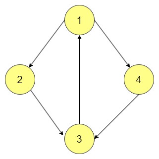
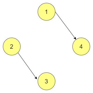
Example
Consider a directed graph G = (V, E) where:
- V is the set of vertices: {1, 2, 3, 4}
- E is the set of directed edges: {(1, 2), (1, 4), (2, 3), (4, 3), (3, 1)}

Key points from the diagram:
- Vertex 1 is connected to 2 and 4.
- Vertices 2 and 4 are both connected to 3.
- Vertex 3 connects back to 1, forming a cycle.

POSTGRADUATE PROGRAM IN
Multi Cloud Architecture & DevOps
Master cloud architecture, DevOps practices, and automation to build scalable, resilient systems.
Common Graph Terminologies
Understanding key terms in graph theory is essential for working effectively with graphs. Below are important terminologies explained.
- Vertex (Node): A point where edges meet. It represents an object or data point.
- Edge: An edge is a line segment joining two vertices indicating the relation existing between the vertices.
- Degree of a Vertex: It describes the number of edges that are connected to a vertex.
- Path: A sequence of edges connecting a series of vertices. Paths show how vertices are related through edges.
- Cycle: A path that starts and ends at the same vertex without repeating any edges or vertices. Cycles are found in cyclic graphs.
- Disconnected Graph: A graph in which at least one pair of vertices has no edge along with a path that connects them. Some vertices are distorted from others.
- Subgraph: A portion of a graph that includes some of its vertices and edges. Subgraphs maintain the connections of the original graph.
- Spanning Subgraph: A spanning subgraph is defined as a subgraph containing all the vertices of the original graph although some analytical edge cannot be included. It contains all the vertices of the graph.
- Connected Component: A maximal connected subgraph. In a disconnected graph, it represents a section where any two vertices are connected by paths.
- Bridge: An edge whose removal increases the number of connected components. It connects two parts of a graph and its absence disconnects the graph.
- Isolated Vertex: A vertex with no edges connected to it. It is not connected to any other vertices.
- Loop: An edge that connects a vertex to itself. Loops are counted twice when calculating the degree of a vertex.
- Parallel Edges: Multiple edges connecting the same pair of vertices. They represent multiple relationships between the same vertices.
- Undirected Graph: In such types of graphs, there is approximately no orientation of the edges. In this case, the relations are not one-directional but are bimodal and edges can be crossed easily in any direction.
- Tree: A connected graph with no cycles. It is minimally connected and has exactly one path between any two vertices.
- Forest: A collection of trees. It is an acyclic graph that may be disconnected.
- Spanning Tree: Subgraph which is a tree and has all the vertices of the previous graph. It unites all points with the least amount of edges.
Types of Graphs in Data Structures
In the case of graphs, there are various types of them, with each having specific attributes which define them in solving various types of issues. Therefore, knowing the common types of graphs is very important in making a decision on the correct method to undertake in accomplishing a particular task.
Simple Graph
A simple graph has no loops (an edge connecting a vertex to itself). It also has no multiple edges between any pair of vertices. There is exactly one edge between any two distinct vertices in the graph.
Example
This graph is a simple graph because:
- Each pair of vertices is connected by only one edge.
- There are no loops, and no multiple edges between any pair of vertices.
Null Graph
A null graph is the simplest type of graph, consisting of a set of vertices without any edges. This means there are no connections between the vertices. Null graphs are often used in theoretical discussions and are not common in practical applications, as there are no relationships to analyse.
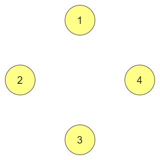
In the above graph, not any single vertex is connected.
Finite Graph
A finite graph contains a limited number of vertices and edges. The set of vertices and edges are both finite, which makes this type of graph suitable for practical applications, such as network analysis, social media graphs, and mapping systems. Most real-world graphs fall into this category.
Infinite Graph
An infinite graph contains an infinite number of vertices, edges, or both. These graphs are used in theoretical computer science and mathematics and are not often found in practical, everyday scenarios. An infinite graph continues endlessly and cannot be fully represented in physical form.
Trivial Graph
A trivial graph consists of just one vertex and no edges.
It is the simplest possible form of a graph and often serves as a theoretical starting point when discussing graph theory. Despite its simplicity, the trivial graph is an important concept in understanding more complex graph structures.
Multi Graph
In the case of multigraphs, there can exist several edges that link up the same pair of vertices. These edges can be different and denote the same vertices with a different relationship. For instance, in the transportation network, many edges exist between the two cities with each edge signifying a different mode of transport.
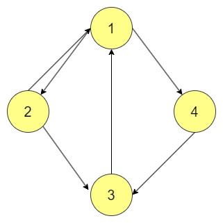
In the above graph, there are 2 edges connecting vertices 1 and 2.
Complete Graph
A complete graph is fully connected, meaning every pair of distinct vertices is connected by a unique edge. It indicates the upper limit of edges that can be achieved for a certain amount of vertices. Complete graphs are efficient in these scenarios because all the elements interact with all other elements.
Pseudo Graph
A pseudograph allows both loops and multiple edges between vertices. A loop is an edge that connects a vertex to itself. This type of graph can model scenarios where entities have complex, multi-layered relationships, such as in social networks with self-connections or repeated interactions.
Subgraph
A subgraph is a smaller portion of a larger graph, consisting of a subset of the original graph’s vertices and edges. Subgraphs must maintain the relationships present in the original graph. They are often used in graph analysis to study specific sections of a larger network.
Regular Graph
A regular graph includes a graph in which each vertex is connected to an equal number of edges implying that each node has the same degree. Regularisation of graphs is often necessary especially when designing a network in which a uniform connection is required. A good example is a peer-to-peer network or distribution of load in balance.
Weighted Graph
In a weighted graph, a numerical value or weight is given to an edge to show its cost, distance or some other relevant dimension. Weighted graphs are often employed in networks in that weight may correlate to distance, travel time or other key elements.
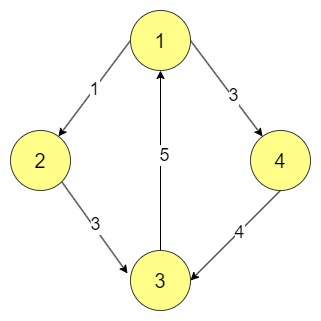
In the above graph, each edge has a particular weight.
Cyclic Graph
A cyclic graph has one or more cycles in it, meaning there is a path that starts from one vertex and comes back to the same vertex. The use of these types of graphs includes the depiction of circulation workflows or recurrent systems where there is a repetitive process or feedback that is exercised.
Acyclic Graph
In an acyclic graph, there are no cycles, that is, no path taken leads back to the initial vertex. These graphs are frequently employed in circumstances that require avoidance of cycles such as in project management where the usage of dependency graph or hierarchy models is in place.
Directed Graph
A directed graph is one in which the edges have a direction, indicating a one-way relationship between vertices. These graphs are used to model processes where order or direction matters, such as in web page links or traffic flow.
Undirected Graph
An undirected graph has edges that do not have a direction, meaning the relationship between any two vertices is bidirectional. This kind of centrality is particularly relevant in graphs which represent properties that are close, like mutual friendships, or networks of roads.
Connected Graph
In a connected graph, there are no pairs of vertices such that no path can traverse from one to the other. To facilitate this, at least, some network properties need to be preserved. Such graphs are very important in representing structures where communication is very critical, for example communication networks.
Disconnected Graph
In graph theory, a disconnected graph has at least one graph component where no edges connect a vertex of that component to any other vertex. This means that some nodes are completely separate from other nodes, and this may be relevant in cases where separation, isolation or partitioning must be represented, for example, partitioned networks, or separated social groups.
In the above diagram, there are 2 graphs.
Representation of Graphs in Data Structures
There are mainly two ways to types of representation of graphs:
- Adjacency Matrix
- Adjacency List
Adjacency Matrix
- An adjacency matrix is a 2D array where rows and columns represent vertices, and the values in the matrix indicate the presence of an edge between the vertices.
- The value is usually 1 (or the edge’s weight) if there is an edge between the vertices, and 0 if there is no edge.
Example
Undirected Graph: As for the case of undirected graphs, the adjacency matrix exhibits a symmetric matrix since the relationship between vertices is not one-sided.
1 1 0
1 0 1
0 1 0
- Here, vertices 1 and 2 are connected, as are vertices 2 and 3.
Directed Graph: For directed graphs, the matrix is not symmetric, as edges have a direction. A value of 1 in the row and column shows the direction from one vertex to another.
0 1 0
0 0 1
0 0 0
- This shows directed edges from 1 to 2 and from 2 to 3.
Weighted Graph: For weighted graphs, the matrix stores the weight of the edge instead of 1.
0 5 0
0 0 3
0 0 0
- This weighted matrix shows a directed edge from 1 to 2 with a weight of 5, and from 2 to 3 with a weight of 3.
Adjacency List
- An adjacency list is a collection of linked lists. The array index represents the vertices and every list in the array stands for the vertices connected to the v-th vertex respectively.
- Each vertex stores a list of all its neighbouring vertices.
- For undirected graphs, both vertices store each other in their lists.
- For directed graphs, only the vertex at the start of the edge stores the destination vertex in its list.
- For weighted graphs, each list entry can store both the adjacent vertex and the weight of the edge.
Example
Undirected Graph:
1: 2
2: 1, 3
3: 2
- This shows vertex 1 connected to 2, and vertex 2 connected to both 1 and 3.
Directed Graph:
1: 2
2: 3
3:
- This list shows vertex 1 has a directed edge to 2, and vertex 2 has a directed edge to 3.
Weighted Graph:
1: (2, 5)
2: (3, 3)
3:
- This shows vertex 1 has a directed edge to vertex 2 with weight 5, and vertex 2 has a directed edge to vertex 3 with weight 3.
Both methods have their own advantages and are chosen based on the needs of the problem, like the number of edges, memory constraints, and the operations performed on the graph.

82.9%
of professionals don't believe their degree can help them get ahead at work.
Operations on Graphs in Data Structures
Graphs require a variety of operations to manage and manipulate the structure. These operations are essential to create, modify, and delete elements in a graph. Below are some key operations commonly performed on graphs.
Creating Graphs
- To create a graph, an empty adjacency matrix (or list) is initialised. The size of the matrix depends on the number of vertices.
- For a graph with n vertices, an n x n matrix is created, filled initially with 0s indicating no edges between vertices.
Example
An adjacency matrix for a graph with 3 vertices:
0 0 0
0 0 0
0 0 0
This represents a graph with 3 vertices and no edges.
Insert Vertex
- To add an additional vertex to the currently existing graph implies extending the existing matrix to form a seat for the new vertex.
- If there are n vertices in the graph, then a new matrix of order (n + 1) x (n + 1) is formed having an additional row and column which is a vector of zeros.
Example
Inserting vertex 4 to an existing graph:
Initial matrix:
0 1 0
1 0 1
0 1 0
Matrix after inserting vertex 4:
0 1 0 0
1 0 1 0
0 1 0 0
0 0 0 0
Now vertex 4 is added but has no edges yet.
Delete Vertex
- In the process of eliminating a vertex, one removes the corresponding row and column of the adjacency matrix.
- Once the deletion is done, the size of the matrix loses one unit in number, which removes edges related to the deleted vertex.
Example
Deleting vertex 2 from the graph:
Initial matrix:
0 1 0
1 0 1
0 1 0
Matrix after deleting vertex 2:
0 0
0 0
Here, vertex 2 and its edges are removed.
Insert Edge
- To insert an edge between two vertices in an adjacency matrix, the corresponding value is updated to 1 (or the weight in case of a weighted graph).
- For undirected graphs, both the symmetric entries in the matrix are updated, while for directed graphs, only one entry is updated.
Example
Inserting an edge between vertex 1 and 3:
Initial matrix:
0 1 0
1 0 1
0 1 0
Matrix after inserting edge between 1 and 3:
0 1 1
1 0 1
1 1 0
This represents an undirected edge between 1 and 3.
Delete Edge
- Deleting an edge involves setting the corresponding matrix value to 0.
- For undirected graphs, both symmetric values are updated to 0, while for directed graphs, only one value is changed.
Example
Deleting the edge between vertex 2 and 3:
Initial matrix
0 1 1
1 0 1
1 1 0
Matrix after deleting edge between 2 and 3:
0 1 1
1 0 0
1 0 0
Here, the edge between 2 and 3 has been removed.
These basic operations form the building blocks for manipulating graph structures and are
widely used in various graph algorithms and applications.
Graph Traversal Algorithm
Graph traversal refers to the visiting process of each vertex of the graph in a systematic manner. Traversal operation ensures that all nodes and edges of the graph have been accessed in order to find an individual node or find every node and executes an operation such as counting, searching or pathfinding.
Here, we have explained Breadth-first search and Depth-first search algorithms with example code to traverse the graph.
Breadth-First Search (BFS)
BFS explores the graph level by level. Starting from a node, it visits all the neighbouring nodes at the present depth before moving on to nodes at the next depth level.
Algorithm Steps
- Begin at a chosen starting vertex, mark it as visited.
- Add the starting vertex to a queue.
- While the queue is not empty:
- Remove the front vertex from the queue.
- Visit all unvisited neighbours of the removed vertex.
- Mark them as visited and add them to the queue.
4. Repeat the process until all vertices are visited.
Python Code
from collections import deque

# BFS function using adjacency matrix

def bfs(graph, start):

visited = [False] * len(graph)  # Keep track of visited vertices

queue = deque([start])  # Initialise the queue with the starting vertex

visited[start] = True  # Mark the starting vertex as visited

while queue:

vertex = queue.popleft()  # Dequeue the front vertex

print(vertex, end=" ")  # Process the vertex (print it here)

# Loop through all vertices to check adjacency

for i in range(len(graph[vertex])):

if graph[vertex][i] == 1 and not visited[i]:  # If there's an edge and the vertex is unvisited

queue.append(i)  # Enqueue the vertex

visited[i] = True  # Mark the vertex as visited

# Example graph as an adjacency matrix

graph = [

[0, 1, 1, 0, 0, 0],  # Edges from vertex 0

[1, 0, 0, 1, 1, 0],  # Edges from vertex 1

[1, 0, 0, 0, 0, 1],  # Edges from vertex 2

[0, 1, 0, 0, 0, 0],  # Edges from vertex 3

[0, 1, 0, 0, 0, 1],  # Edges from vertex 4

[0, 0, 1, 0, 1, 0]   # Edges from vertex 5

]

bfs(graph, 0)  # Start BFS from vertex 0
Java Code
import java.util.*;

public class BFSMatrix {

// BFS function using adjacency matrix

public static void bfs(int[][] graph, int start) {

boolean[] visited = new boolean[graph.length];  // Keep track of visited vertices

Queue<Integer> queue = new LinkedList<>();  // Initialize queue

visited[start] = true;  // Mark the starting vertex as visited

queue.add(start);  // Enqueue the starting vertex

while (!queue.isEmpty()) {

int vertex = queue.poll();  // Dequeue the front vertex

System.out.print(vertex + " ");  // Process the vertex (print it here)

// Loop through all vertices to check adjacency

for (int i = 0; i < graph[vertex].length; i++) {

if (graph[vertex][i] == 1 && !visited[i]) {  // If there's an edge and the vertex is unvisited

queue.add(i);  // Enqueue the vertex

visited[i] = true;  // Mark the vertex as visited

}

}

}

}

public static void main(String[] args) {

// Example graph as an adjacency matrix

int[][] graph = {

{0, 1, 1, 0, 0, 0},  // Edges from vertex 0

{1, 0, 0, 1, 1, 0},  // Edges from vertex 1

{1, 0, 0, 0, 0, 1},  // Edges from vertex 2

{0, 1, 0, 0, 0, 0},  // Edges from vertex 3

{0, 1, 0, 0, 0, 1},  // Edges from vertex 4

{0, 0, 1, 0, 1, 0}   // Edges from vertex 5

};

bfs(graph, 0);  // Start BFS from vertex 0

}

}
Output
0 1 2 3 4 5
Complexity Analysis
- Time Complexity: The time complexity of BFS is O (V + E), where V represents a number of vertices while E represents a number of edges. This is due to the nature of the BFS where every single vertex is visited and all the adjoining edges are covered.
- Space Complexity: The space complexity is O(V) since it deploys a queue that acts as storage of vertices due for processing and also extends a visited array to note out already visited nodes.
Depth-First Search (DFS)
DFS is a graph traversal technique that explores as far down a branch as possible before backtracking. It uses a stack or recursion to keep track of the vertices being visited. DFS is particularly useful for exploring deeper levels of a graph first before moving horizontally across.
Algorithm Steps:
- Start at a chosen vertex and mark it as visited.
- Visit an adjacent unvisited vertex, mark it as visited, and move to this vertex. If there are multiple unvisited neighbours, pick one arbitrarily.
- Repeat step 2 recursively until you reach a vertex with no unvisited adjacent vertices.
- Backtrack to the previous vertex (the last visited vertex with unvisited neighbours) and repeat step 2.
- Continue the process until all vertices in the connected component are visited.
- If any unvisited vertices remain, repeat the process for the next connected component.
DFS explores as deep as possible along a branch before backtracking, which makes it effective for tasks like pathfinding, cycle detection, and topological sorting in directed acyclic graphs (DAGs).
Python Code
# DFS function using adjacency matrix

def dfs(graph, vertex, visited):

visited[vertex] = True  # Mark the current vertex as visited

print(vertex, end=" ")  # Process the vertex (print it here)

# Recursively visit all adjacent vertices

for i in range(len(graph[vertex])):

if graph[vertex][i] == 1 and not visited[i]:  # If there's an edge and the vertex is unvisited

dfs(graph, i, visited)

# Example graph as an adjacency matrix

graph = [

[0, 1, 1, 0, 0, 0],  # Edges from vertex 0

[1, 0, 0, 1, 1, 0],  # Edges from vertex 1

[1, 0, 0, 0, 0, 1],  # Edges from vertex 2

[0, 1, 0, 0, 0, 0],  # Edges from vertex 3

[0, 1, 0, 0, 0, 1],  # Edges from vertex 4

[0, 0, 1, 0, 1, 0]   # Edges from vertex 5

]

visited = [False] * len(graph)  # Initialize visited list

dfs(graph, 0, visited)  # Start DFS from vertex 0
Java Code
public class DFSMatrix {

// DFS function using adjacency matrix

public static void dfs(int[][] graph, int vertex, boolean[] visited) {

visited[vertex] = true;  // Mark the current vertex as visited

System.out.print(vertex + " ");  // Process the vertex (print it here)

// Recursively visit all adjacent vertices

for (int i = 0; i < graph[vertex].length; i++) {

if (graph[vertex][i] == 1 && !visited[i]) {  // If there's an edge and the vertex is unvisited

dfs(graph, i, visited);  // Recursively visit the vertex

}

}

}

public static void main(String[] args) {

// Example graph as an adjacency matrix

int[][] graph = {

{0, 1, 1, 0, 0, 0},  // Edges from vertex 0

{1, 0, 0, 1, 1, 0},  // Edges from vertex 1

{1, 0, 0, 0, 0, 1},  // Edges from vertex 2

{0, 1, 0, 0, 0, 0},  // Edges from vertex 3

{0, 1, 0, 0, 0, 1},  // Edges from vertex 4

{0, 0, 1, 0, 1, 0}   // Edges from vertex 5

};

boolean[] visited = new boolean[graph.length];  // Initialize visited array

dfs(graph, 0, visited);  // Start DFS from vertex 0

}

}
Output
0 1 3 4 5 2
Complexity Analysis
- Time Complexity: The time complexity of DFS is O(V + E) since it traverses all the vertices, visiting all edges in the graph once before finishing the traversal.
- Space Complexity: The space complexity of the DFS method is O(V) is required owing to the recursive stack or explicit stack which is needed in the search of the vertices.
Application of Graphs in Data Structures
Graphs are an important and very versatile structure because they can be applied in any field where relations between discrete objects or entities require modelling and investigation. Here are examples of some of the areas where graphs are applied in data structures:
- Routing Algorithms: Graphs help in representing networks such as roads and the internet where nodes are activities and distant devices while edges are the paths or connections between these nodes.
- Recommendation Systems: Items or users are represented by a vertex and similarity or interaction between them is a connection or an edge.
- Network Flow Analysis: Identification of even a single possible route is done via the usage of graphs representing the flow of data in a circuit.
- Dependency Graphs: When dealing with project management, vertices stand for the activities whereas edges are the links between the activities in terms of their interdependencies.
- Transport Networks: Vertices of such analyses are easily associated with airports, bus or train stations while edges are the routes joining them, thus aiding in the determination of minimum distance or optimum routes taken to reach the specific vertex.
- Web Crawling: The structure of a web can also be mimicked in a graph with web pages as vertices and hyperlinks as edges.
- Circuit Design: A graph in this shows how electrical circuits are interrelated with the nodes, representing the components and the links as the connections.
- Social Networks: In this context, vertices are people while edges demote their connections such as friends, followers or any kind of relationships.
Pros and Cons of Graph Data Structure
Pros
- Scope: Graphs have a considerable range of applications which include social networks, computer networks and transport networks among others.
- Techniques for Better Searching: Properties of graphs make it possible to use effective searching and traversal methods such as BFS and DFS that are important for many problems including shortest-path and connectivity problems.
- Show Connections: Using graphs incorporates all relations among and within entities which suit various problem solving such as in recommendation systems and scheduling.
- Scalable Structure: Graphs can be presented through different forms such as the adjacency matrix and adjacency list, which gives room for varying implementation according to the required solution.
- Graph with Weights: Graphs which incorporate weighted edges make it easy to represent cost, distance or capacity which are important attributes in most optimization problems such as route plan and network flow.
- If Cycle Exists can be Determined: The graphs algorithms have the capacity to discern cycles, this is important in cases such as deadlock detection, etc.
Cons
- High Memory Usage: When using an adjacency matrix format to represent graphs, it can increase the use of memory even in large datasets where the graph is usually sparse.
- Complex Implementation: Working on graphs such as multi-graph and directed, or weighted graphs is complicated and requires sophisticated algorithms and data structures.
- Inefficient for Dense Graphs: Some algorithms for instance the use of adjacency matrix, are not efficient with dense graphs having many edges, because they might have to visit or process all the vertices/edges several times.
- Overhead for Dynamic Operations: These structural modifications like the addition and deletion of vertices and edges are very expensive in terms of time and space, especially in huge complex graphs.
Difference Between Tree and Graph Data Structure
| Feature | Tree | Graph |
| Definition | A tree is a hierarchical data structure where nodes are connected in a parent-child relationship. | A graph is a non-linear data structure consisting of vertices (nodes) and edges that connect them. |
| Structure | A tree is a connected, acyclic graph with a single root node and no loops. | A graph can have cycles, loops, or multiple connections between nodes. |
| Root Node | Trees have a single root node from which all other nodes descend. | Graphs do not have a root node and can have multiple disconnected components. |
| Parent-Child Relationship | In trees, each node (except the root) has exactly one parent, and nodes can have multiple children. | In graphs, there are no strict parent-child relationships; nodes are connected arbitrarily. |
| Direction | Trees are always directed, meaning edges point from parent to child. | Graphs can be directed (edges have direction) or undirected (edges have no direction). |
| Edges | In a tree with n nodes, there are always n-1 edges. | In graphs, the number of edges can vary and is not fixed relative to the number of vertices. |
| Applications | Trees are used in hierarchical structures like file systems, databases, and XML parsing. | Graphs are used in network modelling, social networks, pathfinding, and dependency resolution. |
| Complexity | Trees are simpler, with predictable relationships and traversal methods. | Graphs are more complex due to arbitrary connections and possible cycles. |
Important Graph Algorithms
Graph algorithms provide important solutions to complex problems related to networks, relationships and optimizations faced in modern society. Below are some of the most essential graph algorithms and their respective areas of use or applications.
Depth-First Search (DFS)
- In graph theory, depth-first search is a graph traversal algorithm which means the algorithm moves as far down a branch as possible before backtracking to explore other branches.
- Applications:
- Finding connected components in a graph.
- Detecting cycles in a graph.
- Solving puzzles like mazes.
Breadth-First Search (BFS)
- BFS visits all the nodes at the same level before proceeding to the nodes at a deeper level than the current one.
- Applications:
- Finding the shortest path in an unweighted graph.
- Web crawlers and network broadcast algorithms.
Dijkstra’s Algorithm
- Given a weighted graph, this deals with finding the shortest path between the source and the target nodes.
- Applications:
- Network routing protocols like OSPF.
- Optimising transport networks.
Kruskal’s Algorithm
- Kruskal’s algorithm is also concerned with finding a tree that links all the vertices of a connected graph with the least total edge weight, also known as the Minimum Spanning Tree (MST).
- Applications:
- Clustering in machine learning.
- Network design optimization.
Prim’s Algorithm
- Prim’s algorithm is another algorithm for finding the Minimum Spanning Tree (MST), but within which a Minimum Spanning Tree grows stepwise from one of its odd vertices, by consecutive inclusion of edges.
- Applications:
- Optimising network designs where adding one connection at a time is beneficial.
- Constructing cable or phone networks.
- Power grid design.
Bellman-Ford Algorithm
- The Bellman-Ford algorithm computes shortest paths in a weighted graph, even with negative edge weights.
- Applications:
- Finding the shortest path in graphs with negative weights.
- Detecting negative weight cycles in financial applications.
- Routing in communication networks.
Floyd-Warshall Algorithm
- Floyd-Warshall finds shortest paths between all pairs of nodes in a graph.
- Applications:
- Solving the all-pairs shortest path problem.
- Analysing road networks for shortest travel distances.
- Computing distances in dense graphs.
Topological Sorting
- Topological sorting orders the vertices of a directed acyclic graph (DAG) linearly such that for every directed edge u → v, u comes before v.
- Applications:
- Task scheduling and dependency resolution.
- Determining order of courses in a curriculum with prerequisites.
- Project management (critical path method).
A* Search Algorithm
- A* is a pathfinding algorithm that uses heuristics to efficiently find the shortest path in graphs.
- Applications:
- AI pathfinding in games and robotics.
- Route planning with cost optimization.
- Solving puzzles like the 8-puzzle or Sudoku.
Tarjan’s Algorithm
- Tarjan’s algorithm finds strongly connected components in a directed graph.
- Applications:
- Analysing networks to find clusters.
- Finding components in dependency resolution systems.
- Discovering strongly connected users in social networks.
These algorithms form the backbone of many systems and applications, solving critical problems in areas like networking, pathfinding, and optimization.
Conclusion
Graphs are one of the most universal and common data structures in the field of computer science, and they can represent and address the most complex tasks. As for social networks, routing, or recommendation systems, graphs are efficient for representing and optimising connections between different elements. Containing numerous types, graphs are competent in dealing with both plain and complex associations.
By understanding key graph operations and algorithms like BFS, DFS, and Dijkstra’s algorithm, one can effectively apply graphs to a wide range of applications. The variety of such algorithms makes it possible to effectively solve problems such as finding routes, developing networks for various purposes, scheduling tasks and many others. All set to launch your coding career? Apply for the Hero Vired Integrated Program in Data Science, Artificial Intelligence, & Machine Learning, offered in collaboration with MIT Open Learning.
What is the difference between a tree and a graph?
What is a weighted graph?
What BFS is used for?
What is the purpose of Dijkstra’s algorithm?
What is a connected graph?
What is an adjacency matrix?
Updated on October 16, 2024