
Data structures and algorithms are the foundations of computer science that are commonly used in almost every application when it is developed. Learning data structures and algorithms in Java is a great approach, and can benefit you in various terms.
In this comprehensive guide, we will learn about Data structures and algorithms in Java. We will cover arrays, linked lists, stacks, queues, trees, heaps, etc., data structures using Java, and also learn about various algorithms including searching and sorting.
What is Java?
Java is a high-level, object-oriented programming language. Java is the best choice for programmers to practise the data structures and algorithms, and also do problem-solving questions. Java provides the best in class methods through its Collection Framework. To learn about data structures and algorithms in Java, learn about the time and space complexities also for better understanding.

POSTGRADUATE PROGRAM IN
Multi Cloud Architecture & DevOps
Master cloud architecture, DevOps practices, and automation to build scalable, resilient systems.
What are Data Structures?
Data structures are methods for efficiently accessing and modifying data by efficiently organising and storing it. Programmers can create more effective and streamlined Java programs by having a solid understanding of data structures in the language. Numerous more benefits, such as abstraction and reusability, are provided by data structures. The sort of data being handled and the type of action that must be completed determine which data structure should be used.
Utilising classes and interfaces from the Java Collections Framework, Java defines data structures such as arrays, lists, sets, maps, queues, and stacks. In Java, the ArrayList works as it provides the proper random entry speed, while the LinkedList outperforms the addition and removal processes.
Types of Data Structures
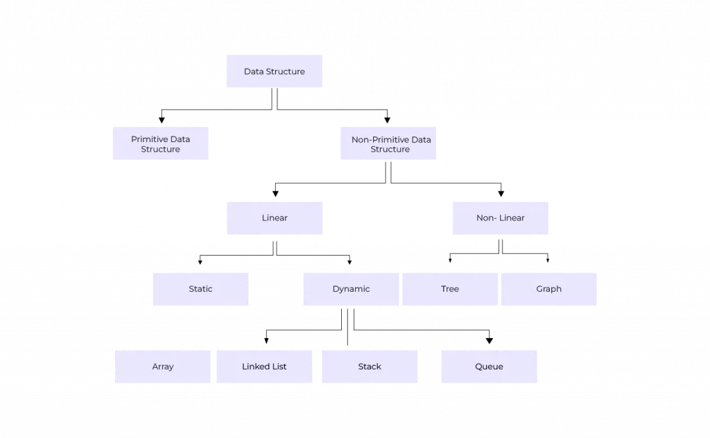
Data structures can be classified into two types:
- Primitive Data Structure
- Non-primitive Data Structure
Primitive Data Structure- The primitive data structures are the fundamental data structures that store values of only one data type—for example, integer, character, float, byte, short, etc.
Non-primitive Data Structure- The non-primitive data structure is then further divided into two types:
- Linear Data Structure
- Non-linear Data Structure
Linear Data Structure
A linear data structure is one in which the data elements are arranged linearly or sequentially, and each element is connected to its previous and next adjacent elements. Arrays, Linked Lists, stacks, queues, and many others are examples of linear data structures.
Linear data structures are further classified as:
- Static Data Structures: These are the static ones that have a set amount of memory. A static data structure’s elements are simpler to access. For example, Arrays.
- Dynamic Data Structures: There is no set size for a dynamic data structure. It can be updated at random while the code is running, which could be regarded as efficient given the code’s complexity in terms of memory and space. For example, Linked List, Stacks, Queues, etc.
Non-linear Data Structure
A non-linear data structure is one in which the data elements are not arranged linearly or sequentially. Here, each element is connected to n-other elements. Examples of non-linear data structures include Trees, Graphs, HashMap, etc.
Array
Arrays are the most basic type of data structure. Elements are stored in contiguous memory locations. Arrays that have a fixed size are often employed when the size of the data is known and does not change dynamically. Using arrays simplifies operations on a whole dataset.
One-dimensional arrays and multi-dimensional arrays are two types of arrays. Elements in an array are the values that are kept there. Indexes are groups of contiguous memory blocks where elements are kept. The amount of elements that make up an array determines its size. For example, arr[] = {1, 2, 3, 4, 5}, specifies the size of arr as 5.
Syntax:
The given below is the syntax used to define an Array in Java:
String[] cars = {“A”, “B”, “C”, “D”};
System.out.println(cars[1]);
// Outputs B
Operations:
The different operations performed by the Array data structure are:
- Access: To access the data elements by their index.
- Update: To change the value of a data element using its index.
- Traversal: To loop through all array elements.
Applications:
The various applications of Arrays are:
- It allows the application of a searching and sorting algorithm.
- Other data structures like stacks, queues, heaps, hash tables, etc. are also implemented using arrays.
- The 2D or matrix problems can also be solved using arrays.
- The CPU can be scheduled using an array.
- The array can be used in computers as a lookup table.
- In image processing, arrays are also used.
- Record administration also makes use of it.
Example: The below example demonstrates the usage of an Array in Java.
public class Main {
public static void main(String[] args) {

// Initialize an array

int[] arr = new int[7];


// Insert elements into the array

arr[0] = 99;

arr[1] = 88;

arr[2] = 77;

arr[3] = 66;

arr[4] = 55;

arr[5] = 44;

arr[6] = 33;


// Accessing elements in the array

System.out.println("Element at index 3: " + arr[3]);

System.out.println("Element at index 4: " + arr[4]);


// Update an element in the array

arr[5] = 43;

System.out.println("Updated element at index 5: " + arr[5]);


// Delete an element from the array (not removing it but setting it to 0 or some value)

arr[3] = 0;

System.out.println("After deletion, element at index 6: " + arr[6]);


// Traverse and print the array

System.out.println("the array elements:");

for (int i = 0; i < arr.length; i++) {

System.out.print(arr[i] + " ");

}

}

}
Output:
Element at index 3: 66

Element at index 4: 55

Updated element at index 5: 43

After deletion, the element at index 6: 33

the array elements:

99 88 77 0 55 43 33
Linked List
A linked list, which is a linear data structure, does not have its items in consecutive memory locations. The linked list’s elements are attached using the pointers. To put it in other words, a Linked List is a linear data structure where the elements are units called nodes that point to each other. By comparison to arrays, linked lists do not have a fixed size.
Syntax:
The given below is the syntax used to define a Linked List in Java:
LinkedList<type> name = new LinkedList<Integer>();
Types of Linked Lists:
The different types of Linked List data structures are:
- Singly Linked List: In this, each node points to the next node.
- Doubly Linked List: In this, each node points to both the next and previous nodes.
- Circular Linked List: In this, the last node or previous node points back to the first node, forming a cycle.
Applications:
The various applications of Linked List are:
- Sparse matrices are represented using a Linked List.
- It is applied to the linked file allocation in the operating system.
- It facilitates memory management in the OS.
- To implement stacks, queues, graphs, etc. using linked lists.
- It is applied to the representation of polynomial manipulation, where a linked list node is represented by each polynomial word.
- It is used as Undo and Redo buttons in browsers
- It is used as the next and previous buttons in image viewer applications.
Example: The below example demonstrates the usage of a Singly Linked List in Java.
class LinkedList {

Node head; // Linked list head


// Linked list node

static class Node {

int data;

Node next;


// Constructor

Node(int d) {

data = d;

next = null;

}

}


// Insert a new node at the end of the list

public void append(int new_data) {

Node new_node = new Node(new_data);


if (head == null) {

head = new_node;

return;

}


Node last = head;

while (last.next != null) {

last = last.next;

}


last.next = new_node;

}


// Insert a new node at the beginning of the list

public void prepend(int new_data) {

Node new_node = new Node(new_data);

new_node.next = head;

head = new_node;

}


// Delete a node by key

public void deleteNode(int key) {

Node temp = head, prev = null;


if (temp != null && temp.data == key) {

head = temp.next;

return;

}


while (temp != null && temp.data != key) {

prev = temp;

temp = temp.next;

}


if (temp == null) return;


prev.next = temp.next;

}


// Print the linked list

public void printList() {

Node tnode = head;

while (tnode != null) {

System.out.print(tnode.data + " ");

tnode = tnode.next;

}

}

}


// Main class

public class Main {


public static void main(String[] args) {

LinkedList ll = new LinkedList();


ll.append(90);

ll.append(80);

ll.append(60);

ll.append(40);

ll.append(20);


System.out.println("Linked list: ");

ll.printList();


System.out.println("\nLinked list after inserting at the beginning: ");

ll.prepend(10);

ll.printList();


System.out.println("\nLinked list after deleting an element: ");

ll.deleteNode(80);

ll.printList();

}

}
Output:
Linked list:

90 80 60 40 20

Linked list after inserting at the beginning:

10 90 80 60 40 20

Linked list after deleting an element:

10 90 60 40 20
Stack
Stacks are the data structures in linear form, which obeys the Last In First Out (LIFO) principle. There is a top, which is the start from where insert (push) and delete (pop) functions are done. A stack can also be used for solving problems, such as deleting the middle element, reversing the stack using recursion, and more. The stack principle is used in daily life.
Syntax: The given below is the syntax used to define a Stack in Java:
Stack<type> st = new Stack<>();
Operations: The different operations performed by the Stack data structure are:
- Push: Add an element to the top of the stack.
- Pop: Remove the topmost element from the stack.
- Peek: View the top element without removing it.
Applications: The various applications of Stack are:
- Operator-and operand-based expressions can be evaluated using a stack.
- For Stacks, it might be a possibility to create a way for backtracking or for checking if the parentheses in an expression match.
- Not only that, but you can also use stacks to change the form of an expression—for instance, infix to postfix, etc.
- It is used for browser history navigation.
- In word processors, the stack is utilised for both undo and redo operations.
- Virtual machines like JVM use the stack.
Example: The below example demonstrates the usage of a Stack in Java.
import java.util.*;

public class Main {

public static void main(String[] args) {

Stack<Integer> st = new Stack<>();

// Push: Adding elements to the stack

st.push(20);

st.push(30);

st.push(50);

System.out.println("Stack after push operations: " + st);


// Pop: Removing elements from the stack

int rem = st.pop();

System.out.println("Removed element: " + rem);

System.out.println("Stack after pop operation: " + st);


// Peek: Get the element at top

int frontElement = st.peek();

System.out.println("Element at the front of the stack: " + frontElement);


// Adding more elements to the stack

st.push(60);

st.push(70);

st.push(80);


// Checking if the stack is empty

boolean chk = st.isEmpty();

System.out.println("Is the stack empty? " + chk);


// Size of the st

int size = st.size();

System.out.println("Size of the stack: " + size);

}

}
Output:
Stack after push operations: [20, 30, 50]

Removed element: 50

Stack after pop operation: [20, 30]

Element at the front of the stack: 30

Is the stack empty? false

Size of the stack: 5
Queue
The queue is a linear data structure that carries out operations in a predetermined order. The data entry placed in the beginning will be reached first, according to the First In First Out (FIFO) order. The removal of items from the rear and insertion of items to the back of the queue are the operations that are being performed. By definition, “enqueue operation” and “dequeue operation” are the terms that are applied when elements are added to and removed from the queue, respectively.
Syntax:
The given below is the syntax used to define a Queue in Java:
Queue<type> que = new LinkedList<>();
Operations:
The Queue data structure carries out various types of operations. Here are a few of them:
- Enqueue: By the enqueue operation, a new element can be added to the end of the queue by turning off the existing elements to the rear.
- Dequeue: Through the dequeue operation, the first element in the queue can be removed from it, therefore being the first also eliminated from a queue.
- Peek: With the peek operation, the front element is to be examined without taking it out of the queue.
- IsEmpty: With the isEmpty operation, the status of the queue can be checked to see if it is empty.
- Size: With the size operation, we can find the number of elements in the queue.
Applications:
The various applications of Queue are:
- Task scheduling (such as queues for printers).
- Handling or responding to queries on web servers.
- It facilitates the preservation of media players’ playlists.
- Queues are used to manage website traffic on a timely basis.
- Operating systems employ queues to handle interrupts.
- Graphs using breadth-first search.
Example: The below example demonstrates the usage of the Queue data structure in Java.
import java.util.*;

public class Main {

public static void main(String[] args) {

Queue<Integer> queue = new LinkedList<>();


// Enqueue: Adding elements to the queue

queue.add(20);

queue.add(30);

queue.add(50);

System.out.println("Queue after enqueue operations: " + queue);


// Dequeue: Removing elements from the queue

int rem = queue.remove();

System.out.println("Removed element: " + rem);

System.out.println("Queue after dequeue operation: " + queue);


// Peek: Get the element at the front of the queue without removing it

int frontElement = queue.peek();

System.out.println("Element at the front of the queue: " + frontElement);


// Adding more elements to the queue

queue.add(60);

queue.add(70);

queue.add(80);


// Checking if the queue is empty

boolean chk = queue.isEmpty();

System.out.println("Is the queue empty? " + chk);


// Size of the queue

int size = queue.size();

System.out.println("Size of the queue: " + size);

}

}
Output:
Queue after enqueue operations: [20, 30, 50]

Removed element: 20

Queue after dequeue operation: [30, 50]

Element at the front of the queue: 30

Is the queue empty? false

Size of the queue: 5
Tree
The tree is a non-linear data structure that contains a hierarchical tree structure. The Tree is a list of nodes where each node contains a value and a pointer reference to the children. Since the tree data structures are non-linear, they provide faster and simpler access to the data. Some of the common names of trees include Node, Root, Edge, Height, Degree, and many more.
Syntax:
The given below is the syntax used to define a Tree in Java:
BinarySearchTree bst = new BinarySearchTree();
Types of Trees:
The different types of Tree data structures are:
- Binary Tree: In this tree, each node would have at most two children.
- Binary Search Tree: It is just another type of a binary tree with ordered nodes.
- AVL Tree: This is a self-balancing binary search tree.
- Red-Black Tree: It is a balanced binary search tree that meets certain properties.
- N-ary Tree: It is a tree that allows having up to n children for each of the nodes.
Applications:
The various applications of Tree are:
- Trees are used in hierarchical data representation like file systems.
- Effective sorting and searching (such as BST).
- A heap is a type of tree data structure used for building priority queues.
- Algorithms for data compression like Huffman coding.
- Database indexing is implemented using B-Tree and B+ Tree.
Example 1: The below example demonstrates the usage of the Binary Tree data structure in Java.
// Define the Node class
class Node {

int data;

Node left, right;


// Constructor to create a new node

public Node(int item) {

data = item;

left = right = null;

}

}


// Define the BT class

class BT {

Node root;


// Constructor

BT() {

root = null;

}


// pre-order traversal

void preOrderTraversal(Node node) {

if (node == null) {

return;

}


System.out.print(node.data + " ");

preOrderTraversal(node.left);

preOrderTraversal(node.right);

}


// in-order traversal

void inOrderTraversal(Node node) {

if (node == null) {

return;

}


inOrderTraversal(node.left);

System.out.print(node.data + " ");

inOrderTraversal(node.right);

}


// post-order traversal

void postOrderTraversal(Node node) {

if (node == null) {

return;

}


postOrderTraversal(node.left);

postOrderTraversal(node.right);

System.out.print(node.data + " ");

}


// BT traversal

void traverse() {

System.out.println("Pre-order traversal:");

preOrderTraversal(root);

System.out.println("\nIn-order traversal:");

inOrderTraversal(root);

System.out.println("\nPost-order traversal:");

postOrderTraversal(root);

}

}


public class Main {

public static void main(String[] args) {


BT tree = new BT();

tree.root = new Node(10);

tree.root.left = new Node(40);

tree.root.right = new Node(50);

tree.root.left.left = new Node(60);

tree.root.left.right = new Node(80);


// Traverse the tree

tree.traverse();

}

}
Output:
Pre-order traversal:

10 40 60 80 50

In-order traversal:

60 40 80 10 50

Post-order traversal:

60 80 40 50 10
Example 2: The below example demonstrates the usage of the Binary Search Tree data structure PreOrder traversal in Java.
// Define the Node class

class TreeNode {

int data;

TreeNode left;

TreeNode right;

// Constructor to create a new node

public TreeNode(int item) {

data = item;

left = right = null;

}

}

// Define the BST class

class BST {

TreeNode root;

// Insert function

public void insert(int data) {

root = insertRec(root, data);

}

// Inserting the data

private TreeNode insertRec(TreeNode root, int data) {

if (root == null) {

root = new TreeNode(data);

return root;

}

if (data < root.data) {

root.left = insertRec(root.left, data);

} else if (data > root.data) {

root.right = insertRec(root.right, data);

}

return root;

}

// pre-order traversal of BST

public void preorderTraversal() {

preorderTraversal(root);

}

// Recursive function for pre-order traversal

private void preorderTraversal(TreeNode root) {

if (root != null) {

System.out.print(root.data + " ");

preorderTraversal(root.left);

preorderTraversal(root.right);

}

}

}


public class Main {

public static void main(String[] args) {

BST bst = new BST();

bst.insert(50);

bst.insert(30);

bst.insert(70);

bst.insert(20);

bst.insert(40);

bst.insert(60);

bst.insert(80);


System.out.print("The preorder traversal of Binary search Tree is: ");

bst.preorderTraversal();

}

}
Output:
The preorder traversal of the Binary Search Tree is: 50 30 20 40 70 60 80Graphs
A graph is a type of non-linear data structure made up of edges (or connections between nodes), and vertices (or nodes). Formally speaking, a graph is made up of a collection of Edges that connect two nodes and a finite number of vertices, also known as nodes.
It uses a variety of terms, such as connected components, adjacent vertices, path, and degree. Examples of Networks, including social networks and transportation systems, are represented by graphs.
Syntax: The given below is the syntax used to define a Graph using an adjacency list in Java: LinkedList<Integer> adj[] // using an adjacency list
Types of Graphs: The different types of Graph data structures are:
- Directed Graph: Edges have a direction.
- Undirected Graph: Edges do not have a direction.
- Weighted Graph: Edges have weights or costs.
- Unweighted Graph: Edges do not have weights.
Operations: The Graph data structure is used for a number of operations. Now let’s look at them.
- DFS (Depth-First Search): A graph can be traversed using a DFS algorithm by reaching the vertices first in depth-first order.
- BFS (Breadth-First Search): In a BFS algorithm, the vertices are visited in a way that lets the graph be traversed in an order.
- Shortest Path: Dijkstra’s algorithm, A* algorithm, and other algorithms can be used to find the shortest path between two vertices.
- Cycle Detection: The method of DFS is used to identify cycles and the means it is believed to be ready in Java programming is the thinking.
Applications: The various applications of Graph are:
- Graphs in Social networks like friend recommendation systems.
- Systems for navigation like, shortest path finding, etc.
- It is applied to graph modelling.
- Resource Allocation Graph is used by the operating system.
- Resolving dependencies like package managers.
Example: The below example demonstrates the usage of Graph data structure using an adjacency list.
import java.util.*;


public class Graph {

private int V;   // No. of vertices

private LinkedList<Integer> adj[]; // Creating an Adjacency List


// Constructor

Graph(int v) {

V = v;

adj = new LinkedList[v];

for (int i = 0; i < v; ++i)

adj[i] = new LinkedList();

}


// Add an edge to the graph

void insertEdge(int v, int w) {

adj[v].add(w);  // Add w to v's list.

}


// Display the adjacency list

void printGraph() {

for (int v = 0; v < V; v++) {

System.out.print("Adjacency list of vertex of graph is: " + v + ": ");

for (Integer node : adj[v]) {

System.out.print(node + " ");

}

System.out.println();

}

}


public static void main(String[] args) {

Graph graph = new Graph(5);


graph.insertEdge(0, 1);

graph.insertEdge(0, 4);

graph.insertEdge(1, 2);

graph.insertEdge(1, 3);

graph.insertEdge(1, 4);

graph.insertEdge(2, 3);

graph.insertEdge(3, 4);


graph.printGraph();

}

}
Output:
Adjacency list of vertex of graph is: 0: 1 5

Adjacency list of vertex of graph is: 1: 2 4 3

Adjacency list of vertex of graph is: 2: 2

Adjacency list of vertex of graph is: 3: 4

Adjacency list of vertex of graph is: 4:
Hash Table
A data structure that maps keys to values for incredibly fast lookup is called a hash table. It transforms keys into indices in an array, where the corresponding values are kept, using a hash function.
Java is a thread-based programming language, therefore HashTable is synchronised and so the thread can only be accessed one at a time thus obtaining thread safety.
By implementing the hashCode and equals methods developers can ensure that the object will be effectively stored and retrieved from the hashtable in Java.
Syntax: The given below is the syntax used to define a Hash Table in Java:
Hashtable<type1, type2> table = new Hashtable<type1, type2>();
Operations: The different operations performed by the Hash Table data structure are:
- Adding Elements: The put() method can be used to add an element to the hashtable.
- Modifying Elements: If we want to modify an element after it has been added, we can do so by adding it again using the put() method.
- Removing Elements: The remove() method can be used to eliminate an element from the Map.
- Traversing Elements: A for loop can be used to iterate the whole hashtable to traverse or print the elements.
Applications:
The various applications of Hash Table are:
- Hashtables are used in the indexing of databases.
- Data caching i.e., the memorization in dynamic programming
- Hashtables are used in counting frequencies, such as the number of times a term appears. It is useful in competitive problem-solving.
Example: The below example demonstrates the usage of the Hashtable data structure in Java.
import java.util.*;

public class Main {

public static void main(String[] args) {

// Creating a Hashtable

Hashtable<String, Integer> myNum = new Hashtable<>();


// Adding key-value pairs to the Hashtable

myNum.put("First", 1);

myNum.put("Second", 2);

myNum.put("Third", 3);

myNum.put("Fourth", 4);

myNum.put("Fifth", 5);


// Display the elements of the Hashtable

System.out.println("Hashtable: " + myNum);


// Accessing a value using the key

System.out.println("The value associated with key 'Fifth': " + myNum.get("Fifth"));


// Remove a key-value pair

myNum.remove("Three");


// Display the Hashtable after removing a key-value pair

System.out.println("After removing 'Two': " + myNum);


// Check if a key exists

System.out.println("Does key 'Fifth' exist? " + myNum.containsKey("Fifth"));


// Traversing the Hashtable

Enumeration<String> keys = myNum.keys();

System.out.println("Iterating over Hashtable:");

while (keys.hasMoreElements()) {

String key = keys.nextElement();

System.out.println(key + " -> " + myNum.get(key));

}

}

}
Output:
Hashtable: {Fifth=5, Second=2, Fourth=4, First=1, Third=3}

The value associated with key 'Fifth': 5

After removing 'Two': {Fifth=5, Second=2, Fourth=4, First=1, Third=3}

Does key 'Fifth' exist? true

Iterating over Hashtable:

Fifth -> 5

Second -> 2

Fourth -> 4

First -> 1

Third -> 3
Heaps
Heap is a unique type of tree-based data structure that complies with the heap property. It is a complete binary tree that makes up the tree in a heap. It is helpful for Heap Sort algorithms and can be used to implement priority queues.
Syntax: The given below is the syntax used to define a Heap in Java:
PriorityQueue<type> pq = new PriorityQueue<>(); // Min-heap
Types of Heaps:
There are two types of heap data structures:
- Max-heap: The root node in this heap needs to have the highest value out of all of its child nodes, and the same goes for its left and right sub-trees. It can be implemented using PriorityQueue in Java.
- Min-heap: The root node in this heap needs to have the lowest value out of all of its offspring nodes, and the same goes for its left and right sub-trees. It can be implemented using PriorityQueue in Java. Min-heap is the default heap when declared.
Applications:
The various applications of Heap are:
- The heap data structure is used in priority queues.
- It is used in Dijkstra’s algorithm for graphs.
- The heap sort algorithm is another application for sorting.
Example 1: The below example demonstrates the usage of a heap data structure for Max-heap using PriorityQueue.
import java.util.*;


public class Main {

public static void main(String[] args) {

// Max Heap (Using custom comparator for descending order)

PriorityQueue<Integer> maxHeap = new PriorityQueue<>(Collections.reverseOrder());


maxHeap.add(34);

maxHeap.add(76);

maxHeap.add(89);

maxHeap.add(23);


System.out.println("Max Heap:");

while (!maxHeap.isEmpty()) {

System.out.println(maxHeap.poll()); // Remove and print elements in descending order

}

}

}
Output:
Max Heap:

89

76

34

23
Example 2: The below example demonstrates the usage of a heap data structure for Min-heap using custom heap implementation.
import java.util.*;


public class Main {

public static void main(String[] args) {

// Min Heap

PriorityQueue<Integer> minHeap = new PriorityQueue<>();


minHeap.add(34);

minHeap.add(76);

minHeap.add(89);

minHeap.add(23);


System.out.println("Min Heap:");

while (!minHeap.isEmpty()) {

System.out.println(minHeap.poll()); // Remove and print elements

}

}

}
Output:
Min Heap:

23

34

76

89
Example 3: The below example demonstrates the usage of a heap data structure for Max-heap using custom heap implementation.
import java.util.*;


public class MaxHeap {

private int[] heap;

private int size;

private int maxSize;


public MaxHeap(int maxSize) {

this.maxSize = maxSize;

this.size = 0;

this.heap = new int[maxSize + 1];

this.heap[0] = Integer.MAX_VALUE;

}


private int parent(int pos) { return pos / 2; }

private int leftChild(int pos) { return 2 * pos; }

private int rightChild(int pos) { return 2 * pos + 1; }

private boolean isLeaf(int pos) { return pos >= (size / 2) && pos <= size; }


private void swap(int fpos, int spos) {

int tmp;

tmp = heap[fpos];

heap[fpos] = heap[spos];

heap[spos] = tmp;

}


private void maxHeapify(int pos) {

if (isLeaf(pos)) return;


if (heap[pos] < heap[leftChild(pos)] || heap[pos] < heap[rightChild(pos)]) {

if (heap[leftChild(pos)] > heap[rightChild(pos)]) {

swap(pos, leftChild(pos));

maxHeapify(leftChild(pos));

} else {

swap(pos, rightChild(pos));

maxHeapify(rightChild(pos));

}

}

}


public void insert(int element) {

heap[++size] = element;

int current = size;


while (heap[current] > heap[parent(current)]) {

swap(current, parent(current));

current = parent(current);

}

}


public int extractMax() {

int popped = heap[1];

heap[1] = heap[size--];

maxHeapify(1);

return popped;

}


public static void main(String[] args) {

MaxHeap maxHeap = new MaxHeap(10);

maxHeap.insert(34);

maxHeap.insert(76);

maxHeap.insert(89);

maxHeap.insert(67);

maxHeap.insert(44);

maxHeap.insert(23);


System.out.println("The max value is " + maxHeap.extractMax());

}

}
Output:
The max value is 89
Example 4: The below example demonstrates the usage of a heap data structure for Min-heap using PriorityQueue.
import java.util.*;


public class MinHeap {

private int[] heap;

private int size;

private int maxSize;


public MinHeap(int maxSize) {

this.maxSize = maxSize;

this.size = 0;

this.heap = new int[maxSize + 1];

this.heap[0] = Integer.MIN_VALUE;

}


private int parent(int pos) { return pos / 2; }

private int leftChild(int pos) { return 2 * pos; }

private int rightChild(int pos) { return 2 * pos + 1; }

private boolean isLeaf(int pos) { return pos >= (size / 2) && pos <= size; }


private void swap(int fpos, int spos) {

int tmp;

tmp = heap[fpos];

heap[fpos] = heap[spos];

heap[spos] = tmp;

}


private void minHeapify(int pos) {

if (isLeaf(pos)) return;


if (heap[pos] > heap[leftChild(pos)] || heap[pos] > heap[rightChild(pos)]) {

if (heap[leftChild(pos)] < heap[rightChild(pos)]) {

swap(pos, leftChild(pos));

minHeapify(leftChild(pos));

} else {

swap(pos, rightChild(pos));

minHeapify(rightChild(pos));

}

}

}


public void insert(int element) {

heap[++size] = element;

int current = size;


while (heap[current] < heap[parent(current)]) {

swap(current, parent(current));

current = parent(current);

}

}


public int extractMin() {

int popped = heap[1];

heap[1] = heap[size--];

minHeapify(1);

return popped;

}


public static void main(String[] args) {

MinHeap minHeap = new MinHeap(10);

minHeap.insert(34);

minHeap.insert(76);

minHeap.insert(89);

minHeap.insert(67);

minHeap.insert(44);

minHeap.insert(23);


System.out.println("The max value is " + minHeap.extractMin());

}

}
Output:
The max value is 23
What is an Algorithm?
Algorithms are sets or equations that use certain steps to solve problems. Algorithms are a foundational feature of computer science. An important aspect for individuals to learn data structures and algorithms is the solid foundational knowledge of algorithms.
How does an Algorithm Work?
Algorithms are the step-by-step process of doing something. Generally, algorithms adhere to a logical structure.
- Data: It is the data that the algorithm takes as input.
- Processing: The input data is subjected to some procedures by the algorithm.
- Output: The intended output generated by the algorithm.
Types of Algorithms
Different types of algorithmic strategies are needed to tackle different kinds of issues most efficiently. Java provides different algorithms to use in their language to create different programs. Although there are many different kinds of algorithms, the most crucial and fundamental ones that you need to know about are covered here.
Searching Algorithms
Searching algorithms are the algorithms that are used to do searches in the data elements. The process of searching involves looking for the required element within a collection of data elements. The following are some typical searching algorithms that are most commonly used:
1. Linear Search
Linear search, which is the most basic search method, is often called sequential search. This searching strategy examines the set of elements one by one and thus uses an iterative or repeated computation. In case the targeted element is found, the address of the target is returned and if it is not found, null is returned.
Example:
public class Main {

public static int linearSearch(int[] arr, int target) {

for (int i = 0; i < arr.length; i++) {

if (arr[i] == target) {

return i; // Target found, return index

}

}

return -1; // Target not found, return -1

}


public static void main(String[] args) {

int[] numbers = {33, 44, 55, 66, 77, 88};

int target = 77;


int ans= linearSearch(numbers, target);

if (ans != -1) {

System.out.println("Target element found at index: " + ans);

} else {

System.out.println("Target element not found in the array.");

}

}

}
Output:
Target element found at index: 4
2. Binary Search
Binary search is a smart search algorithm in Java that will look for a target element by dividing the search space into halves. It operates by continually dividing the search interval in half until the target value is either discovered or the interval becomes empty.
Binary search is a smart search algorithm in Java that will look for a target element by dividing the search space into halves. It operates by continually dividing the search interval in half until the target value is either discovered or the interval becomes empty.
Example:
public class Main {

public static int binarySearch(int[] arr, int target) {

int left = 0, right = arr.length - 1;

while (left <= right) {

int mid = left + (right - left) / 2;


// Check if target is present in mid

if (arr[mid] == target)

return mid;


// If the target is greater, ignore the left half

if (arr[mid] < target)

left = mid + 1;


// If the target is smaller, ignore the right half

else

right = mid - 1;

}


// Target element not present

return -1;

}


public static void main(String[] args) {

int[] arr = {22, 33, 44, 55, 66, 77};

int ans = binarySearch(arr, 55);

if (ans == -1)

System.out.println("Target element not found");

else

System.out.println("Target element found at index " + ans);

}

}
Output:
Target element found at index 3
Sorting Algorithms
Sorting algorithms are used to sort the data elements. Sorting algorithms are capable of sorting the data either in ascending or descending order. It is also employed to efficiently and effectively arrange data. The two most common types of ordering are lexicographical and numerical. The sorting algorithms bubble sort, insertion sort, merge sort, selection sort, and bucket sort are a few examples of frequent problems that can be resolved. The following are some typical searching algorithms that are most commonly used:
1. Bubble Sort
Bubble sort is referred to as the simplest sorting algorithm. It works by comparing each element in the list with the one next to it. These comparisons continue until the whole array is properly ordered. Easy to program and understand, bubble sort proves inefficient for large datasets. The time complexity is O(n^2) for both average and worst cases. Its simplicity is at the core of what makes it advantageous, coupled with performance limitations that prohibit large-scale use.
Example:
public class Main {

public static void bubbleSort(int[] arr) {

int n = arr.length;

for (int i = 0; i < n - 1; i++) {

boolean swapped = false;

for (int j = 0; j < n - i - 1; j++) {

if (arr[j] > arr[j + 1]) {

// Swap arr[j] and arr[j + 1]

int temp = arr[j];

arr[j] = arr[j + 1];

arr[j + 1] = temp;

swapped = true;

}

}

// If no two elements were swapped in the inner loop, the array is sorted

if (!swapped) {

break;

}

}

}


public static void main(String[] args) {

int[] numbers = {64, 34, 25, 12, 22, 11, 90};


System.out.println("Original array:");

printArray(numbers);


bubbleSort(numbers);


System.out.println("Sorted array:");

printArray(numbers);

}


public static void printArray(int[] arr) {

for (int num : arr) {

System.out.print(num + " ");

}

System.out.println();

}

}
Output:
Original array:

64 34 25 12 22 11 90

Sorted array:

11 12 22 25 34 64 90
2. Insertion Sort
Insertion sort, a simple algorithm, is a step-by-step procedure to sort an array in its appropriate order. This is accomplished by continually taking the next unsorted element and inserting it into its proper place within the already sorted section. The time complexity of this sorting algorithm is O(n^2) both in the worst and average cases. The insertion sort stands no chance of being applied to big instances but it is highly efficient with small and nearly sorted arrays. The insert-itself method is highly effective in the case of small lists and is often used as a supporting route in more complicated algorithms such as quick sort.
Example:
public class insertion {

public static void main(String[] args) {

int[] arr= {7, 23 ,12, 44 ,2, 45};

insertionSort(arr);

for(int num : arr) {

System.out.print(num + " ");

}

}


// [7, 23 ,12, 44 ,2, 45]

static void insertionSort(int[] arr) {

int n = arr.length;

for(int i = 0; i < n-1; i++) {

int j = i;

while(j > 0 && arr[j-1] > arr[j]) {

swap(arr, arr[j-1], arr[j]);

j--;

}

}

}


static void swap(int[] arr, int f, int l) {

int temp = arr[f];

arr[f] = arr[l];

arr[l] = temp;

}

}
Output:
2, 7, 12, 23, 44, 45
3. Selection Sort
Selection sort works by taking up the division of the array into sorted and unsorted portions. It then finds the smallest (or largest) element from the unsorted part and swaps it with the first element in the unsorted part. The process repeats itself, thus steadily expanding the sorted part.
Asymptotically, at 0(n^2) time complexity, selection sort is more efficient than bubble sort in some cases for small datasets but still less ideal for big datasets. It is typically used when memory writes are very expensive because it minimises swapping (n-1) times.
Example:
public class selection {

public static void main(String[] args) {

int[] arr = { 4, 512, 12, 55, 134, 4 };


selSort(arr);

for(int num : arr) {

System.out.print(num + " ");

}

}


static void selSort(int[] arr) {

for(int i = 0; i < arr.length - 1; i++) {

int maxIndex = getMax(arr, i);

swap(arr, i, maxIndex);

}

}


static int getMax(int[] arr, int start) {

int maxIndex = start;

for(int i = start + 1; i < arr.length; i++) {

if(arr[i] > arr[maxIndex]) {

maxIndex = i;

}

}

return maxIndex;

}


static void swap(int[] arr, int i, int j) {

int temp = arr[i];

arr[i] = arr[j];

arr[j] = temp;

}

}
Output:
512 134 55 12 4 4
4. Quick Sort
Quick sort is a comparison sort, dividing the array into two partitions first, and then using a recursive approach to sort all of them. It sorts by selecting a pivot and then identifying the partitioning index; the left side of the partition is less than or equal to the selected pivot (arr[pivot]) element.
The time complexity for Quick Sort on average is O(n log n), it is not stable since it does an in-place comparison sort. This property of Quick Sort makes it suitable for large datasets. It has an in-place space complexity of O(log n).
Example:
public class quicksort {

public static void main(String[] args) {

int[] num = { 5, 34, 233, 3, 13, 5, 0 };

qs(num, 0, num.length-1);

for(int i = 0; i < num.length; i++) {

System.out.print(num[i] + " ");

}

}


static void qs(int[] arr, int low, int high) {

if(low < high) {

int partition = partition(arr, low, high);

qs(arr, low, partition - 1);

qs(arr, partition + 1, high);

}

}


static int partition(int[] arr, int low, int high) {

int pivot = arr[low];

int i = low;

int j = high;


while(i < j) {

//go on till finding the first element greater than pivot

while(arr[i] <= pivot && i <=high - 1) {

i++;

}


the //go on till finding the first element smaller than pivot

while(arr[j] > pivot && i >= low + 1) {

j--;

}


ithe f(i < j) {

int temp = arr[i];

arr[i] = arr[j];

arr[j] = temp;

}

}

int temp = arr[low];

arr[low] = arr[j];

arr[j] = temp;

return j;

}

}
Output:
0 3 5 5 13 34 233
5. Merge Sort
Merge sort is a divide-and-conquer algorithm that divides the array into two halves. It then recursively sorts each half of the list and, in the process of merging the second half, merges the sorted halves. Merge sort has a time complexity of O(n log n) in all cases. It is very efficient and stable; thus, it is an appropriate program for very large datasets. This is because it takes up extra space that is proportionate to the size of the array to be sorted.
Example:
public class MergeSort {

public static void main(String[] args) {

int n = 7;

int[] num = { 5, 34, 233, 3, 13, 5, 0 };

mergeSort(num, 0, n - 1);

for(int i = 0; i < n; i++) {

System.out.print(num[i] + " ");

}

}


static void mergeSort(int[] arr, int low, int high) {

if(low >= high) return;

int mid = (low+high) / 2;


mergeSort(arr, low, mid);

mergeSort(arr, mid+1, high);

merge(arr, low, mid, high);

}


static void merge(int[] arr, int low, int mid, int high) {

ArrayList<Integer> temp = new ArrayList<>();

int left = low;

int right = mid + 1;


while(left <= mid && right <= high) {

//comparison

if(arr[left] < arr[right]) {

temp.add(arr[left]);

left++;

} else {

temp.add(arr[right]);

right++;

}

}


while(left <= mid) {

temp.add(arr[left]);

left++;

}


while(right <= high) {

temp.add(arr[right]);

right++;

}


for(int i = low; i <= high; i++) {

arr[i] = temp.get(i - low);

}

}

}
Output:
0 3 5 5 13 34 233
Recursive Vs Iterative Approaches in Algorithms
In Java, you can write and run an algorithm either recursively or iteratively. Both have their pros and cons depending on the situation, specific problem, and given constraints. Let’s see how they both differentiate and learn about their syntax, examples, and more.
Recursive Approach
Recursion is a technique where the function calls itself within its body to split the problem into smaller, more manageable sub-problems. Recursion might be defined more simply as the process by which a function repeatedly calls itself. It is especially helpful for issues that can be divided into more manageable, related sub-issues.
Syntax:
int functionName(parameter) {
return functionName(); // recursive call
}
Example:
int factorial(int num) {

if (num == 0) return 1;

return num * factorial(num - 1);

}
This is a simple recursive algorithm in Java that finds the factorial of a number (num) and returns it. As you can see the function factorial() takes num as an argument, and returns the factorial of it by recursive function call.
Iterative Approach
Iteration is a method that runs a code block repeatedly up until the condition is not met. The most common way to construct it is with loops (for, while, do-while).
Syntax:
int functionName(parameter) {
// you code goes here
return n;
}
Example:
int findFactorial(int num) {

int ans = 1;

for (inYour= 2; i <= num; i++) {

ans *= i;

}

return ans;

}
This is a simple iterative algorithm in Java to find the factorial of a number (num) and return it. As you can see the function findFactorial() takes num as an argument, and runs a for loop to calculate the factorial of the num.
Algorithm Complexity and Big O Notation
When we talk about algorithm complexity, it means finding out the time and space complexity of an algorithm. It is necessary to comprehend algorithm complexity to write effective code. Big O notation is the most often used term for time and space complexity. Algorithms that solve the same problem more quickly and with less space should be chosen over those that do it more slowly and use more space.
What is a Big O Notation?
In complexity theory, computer science, and mathematics, the symbol “Big O” is used to represent the asymptotic behaviour of functions. In essence, it indicates the rate at which a function increases or decreases. A mathematical notation known as “Big O” is used to express the top bound of an algorithm’s worst-case space or running time needs. It offers a broad understanding of how the performance of the algorithm changes with the size of the input.
What Makes Big O Important?
Big O notation makes it easier for programmers to comprehend how their algorithms will function as the size of the input rises. Better code optimization is made possible by this understanding, particularly in situations where performance is crucial. It also offers a means of contrasting various algorithms for the same problem.
What is a Space Complexity?
In addition to time complexity, algorithms also incorporate space complexity: it quantifies the amount of memory that will be consumed by the method as a function of input size. The notation is also used to specify big O space complexity. This is vital for algorithms processing large data sets or those running on memory-constrained environments.

82.9%
of professionals don't believe their degree can help them get ahead at work.
Advantages of Data Structures in Java
Java offers several advantages for doing data structures and algorithms, and some of them are:
- Rich Collections Framework
Java offers a robust collections framework that includes interfaces and classes for a variety of data structures, making it easy to implement and switch between different structures as needed. Java’s generics enable type-safe data structures, reducing runtime errors and increasing code reliability.
- Built-in Synchronisation
Vector and Hashtable are legacy data structures that are thread-safe, which is a key attribute for them as they can be used in concurrent environments without additional synchronisation mechanisms.
- Efficiency in Storage and Retrieval
Arrays offer constant-time access to elements by index, making them ideal for situations where you need quick lookups. The HashMap in Java provides average-case constant-time complexity O(1) for insertions, deletions, and lookups, making it extremely efficient for associative data storage.
- Versatility
ArrayList – a dynamic resizing allows it to handle varying data sizes, unlike fixed-size arrays. LinkedList is efficient in scenarios where frequent insertions and deletions are needed, particularly at the beginning or end of the list.
- Simplified Data Management
Stack and Queue provide structured data management for Last-In-First-Out (LIFO) and First-In-First-Out (FIFO) operations, respectively, making them useful in algorithms like depth-first search or breadth-first search.
Tree like Binary Search Tree allow hierarchical data representation, which is beneficial in scenarios like representing organisational structures or performing range queries.
Disadvantages of Data Structures in Java
While Java provides several advantages, there are some disadvantages also, and here are some of them:
- Performance Overhead
Apart from the fact that Java brings type safety, generics can still overload the system by taking over the memory of the program in the runtime, for there is type erasure going on at this stage which requires extra casting. Garbage collection is often related to excessive latency which might lead to decreased performance, especially in real-time systems. - Memory Fragmentation
Java’s dynamic memory allocation for data structures such as LinkedLists and ArrayLists can cause memory fragmentation over time. This can have an impact on performance, particularly in programs that operate for extended periods. - Primitive Data Handling Issues
Primitive data handling is rigid because Java’s data structures work with objects and require the usage of wrapper classes for primitive types (such as Integer for int), which can add needless cost and memory usage. Autoboxing/unboxing, the automatic conversion between primitives and their wrapper classes, can cause subtle performance problems, especially in tight loops. - Lack of Resources
Within functional programming paradigms, where immutability is encouraged for safer code, the absence of built-in support for immutable data structures might be a drawback.
Memory Management in Java
Understanding how Java manages memory is crucial for writing efficient and memory-safe applications that use data structures and algorithms.
Understanding Heap Memory in Java
The runtime data space known as the heap is where all class instances and arrays get their memory allocation from. The actual objects are kept in a heap. It is created at the beginning of the JVM. If necessary, the user can manage the heap. Its size might be either fixed or variable. The JVM generates an instance of the object in a heap when you use a new keyword. As that object’s reference is stored in the stack. Every JVM process that is currently executing has a single heap. Garbage is collected when the heap is filled.
Understanding Stack Memory in Java
Local variables and function call frames are kept in the stack memory. In Java, every thread has its stack that runs according to the principle of last-in, first-out, or LIFO. Its size might be either dynamic or fixed. Memory for the stack is allotted to each thread. Partial findings and data are stored in it. It has heap object references in it. Additionally, it contains the value itself rather than a heap-based object reference.
Garbage Collection in Java
The process of automatically identifying and recovering memory that the program is no longer using is known as garbage collection in Java. The tool that performs this process is known as a Garbage Collector (GC). Garbage collection enhances the performance of the application and stops memory leaks.
Working of Garbage Collection:
- When an object is out of the application’s grasp, the garbage collector (GC) recognizes it automatically.
- These items’ memory is detected, at which point it is released for further usage.
- The JVM controls the frequency and functionality of the GC, which operates in the background.
Conclusion
In this comprehensive guide, we have covered the complete data structures and algorithms in Java for beginners. We have learned about various data structures such as arrays, linked lists, stacks, queues, trees, graphs, etc. To assist you gain practical experience with these foundational concepts, each topic contains the code examples along with their outputs.
What are data structures and algorithms in Java?
Does Java provide a collection framework like in C++?
How much Java is required to learn DSA?
What are some common data structures and algorithms in Java?
What is the time and space complexity of the algorithm in Java?
Updated on September 6, 2024