
One of the fundamental aspects of Artificial intelligence is the Constraint Satisfaction Problem (CSP) which represents a class of problems that are specifically solved with the help of reducing constraints or those problems having too many variables. CSPs play a very important role in solving scheduling problems, puzzle-solving problems, and map colouring. The main aim is to divide any complex problem into small possible outcomes based on constraints and reach the optimised solution using backtracking. Hence, CSPs provide a structured framework for handling complex problems and decision-making for the AI model.
In this post, we will discuss how CSP algorithms work with different techniques and discuss different CSP examples like sudoku solver, graph colouring, etc. This will give you an overall idea of the flow of working for CSPs.
Constraint Satisfaction Problem in AI
CSPs are structured around three main components, which help divide the problem and build a solution by reducing the number of total possible variables or probable moves in a game. The three components are Variables, Domains, and Constraints. Let’s look at each component and its role in CSPs.
Variables
Variables work to represent any specific entity that needs to be assigned a value in a problem. Just like we need variables in a scheduling problem to represent time slots, tasks, resources, users, etc. Variables are the total number of resources available to us. In CSP, variables are denoted by X = {X1, X2, …, Xn}.
Domains
Each variable in CSP must have its own corresponding domain, which helps to denote the set of total possible values that the variable can take. The domain of any variable Xi is denoted by Di. For example, we take the same scheduling problem and we take the time slot as variable V1. Then this variable must have the domain of 24 hours (precision can be taken up to hours, minutes or seconds, etc.) denoted by D1.
Constraints
Finally, constraints define the relationship between different variables so that we can restrict the total number of variables by defining a contradicting situation or value. There are a few types of constraints:
- Unary Constraint: These can only involve a single variable, which will restrict the domain of that variable. A specific task or any independent variable in any puzzle can be an unary constraint,
- Binary Constraint: These constraints have the inclusion of pairs of variables and the whole pair is taken as one. Then the combined domain of pairs of variables is reduced. For example, colouring problems in maps, where pairs of vertex points can be taken.
- Higher-order Constraints: Involve three or more variables and together impose restrictions on their collective values. It can be helpful in defining a sum of values assigned to a set of variables and other complex problems.

POSTGRADUATE PROGRAM IN
Data Science & AIML
Learn Data Science, AI & ML to turn raw data into powerful, predictive insights.
Representation of Constraint Satisfaction Problems (CSPs)
CSPs can be represented mathematically using sets, functions and logical expressions.
Formally, a CSP is defined by a triple (X, D, C):
- X: Finite set of variables: X = {X1, X2, …, Xn}.
- D: Set of domains: D = {D1, D2, …, Dn} where Di is the domain of Xi.
- C: Set of constraints: C = {C1, C2, …, Cm}. Cj is a subset of variables with some relation between those variables.
Example of CSP:
Let’s take one famous problem, the N-Queens Problem, which involves placing N queens on the NxN chessboard so that no two queens threaten each other. Hence, no two queens can share the same row, column or diagonal. Therefore, we define constraints like:
- Variables: X = [Q1, Q2, …, Qn]
- Domains: Di = {1, 2, …, N}
- Constraints: No two queens can be in the same row: Qi ≠ Qj for all i ≠ j. Also, queens cannot be on the same diagonal. Hence for major and minor diagonal: |Qi – Qj| ≠ |i-j| for all i ≠ j, and
CSP Solving Techniques
- Backtracking: It is a depth-first-search algorithm that investigates the previous search space of possible solutions until and unless an optimised solution is found. This is a recursive process and includes going back up to one space and checking for possible solutions.
- Advanced Backtracking: This is similar to a normal backtracking algorithm but it involves direct backtracking to the potential issued outcome. Hence it saves many more operations than normal backtracking.
- Constraint Propagation: This technique reduces the overall search space by enforcing local consistency properties. Hence, it helps detect and eliminate inconsistent values only in the early phase.
- Local Search Algorithms: This includes many algorithms like Hill Climbing, Simulated Annealing, Genetic Algorithms, etc. which can explore the space of possible variable assignments by improving a complete assignment iteratively.
Constraint Satisfaction Problem Algorithm & Implementation
Any CSP-solving approach involves the inclusion of a backtracking algorithm which hits depth-first-search, seeing all possible outcomes and backtracking to wherever there is a locked situation. When we combine depth-first-search with constant propagation, we can highly improve the efficiency of the model. An algorithm for finding solutions for map conditions using nodes and graph edges is given below.
Algorithm:
- Variable Selection: The variable that has not been assigned a value.
- Choose Value: Choose any domain value of that variable
- Check Consistency: Checking any violating constraints
- Constraint Satisfied: If it is consistent, continuously assign the value and attempt to assign the next remaining values
- Not Satisfied: Or else if not consistent or the recursive call fails, then backtrack. Remove the value assignment and try the next value
- Recursion: Repeat until all the variables are assigned and no variable remains without violating constraints.
Code:
class CSP:

def __init__(self, variables, domains, constraints):

self.variables = variables

self.domains = domains

self.constraints = constraints

self.keeptrack = {}

def is_consistent(self, var, value):

for (neighbour, constraint) in self.constraints[var]:

if neighbour in self.keeptrack and not constraint(value, self.keeptrack[var2]):

return False

return True

def select_unassigned_variable(self):

for var in self.variables:

if var not in self.keeptrack:

return var

return None

def backtracking_search(self):

return self.backtrack()

def backtrack(self):

if len(self.keeptrack) == len(self.variables):

return self.keeptrack

var = self.select_unassigned_variable()

for value in self.domains[var]:

if self.is_consistent(var, value):

self.keeptrack[var] = value

result = self.backtrack()

if result:

return result

del self.keeptrack[var]

return None
Explanation:
Here, the CSP Class represents a Constraint Satisfaction Problem with several functions and a backtracking algorithm. The functions are:
- ‘__init__’: This initialises variables, domains, and constraints that we assign during calling the main class function. An empty dictionary, ‘keeptrack’ is used to keep track of assigned variables.
- ‘is_consistent’: This function checks all the constraints by comparing values of neighbour elements in a map.
- ‘select_unassigned_variable’: Utilises the ‘variables’ and selects an unassigned variable from it that runs until all the variables are assigned.
- ‘backtrack’: The main backtracking algorithm for the code includes base case conditions, followed by variable selection, try values, consistency check, and the removal of empty solution and recursive backtrack call until the true solution is found.

82.9%
of professionals don't believe their degree can help them get ahead at work.
Map Colouring Problem
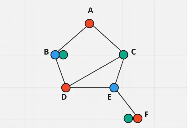
Here, you can see a graph representing six vertices with seven edges, given a total number of colours equal to three, i.e. red, green and blue. The main goal is to assign these three colours across all vertices so that none of the same colours come in adjacent vertices.
To solve this problem using CSP, we first define variables, domains and constraints.
Consider an example of a Map Colouring Problem solved using CSP. The main goal while colouring the map is to ensure that no adjacent regions can have the same colour. Consider a small map with 4 vertices. Hence, the graph can be represented as:
Nodes: A, B, C, D, E, F
Edges: (A, B), (A, C), (B, D), (C, D), (D, E), (C, E), (E, F)
Variables: Each region on the map can be a variable. Here X = {A, B, C, D}
Domains: Possible colours for each region. Di = DA = DB = DC = DD = {Red, Green, Blue}.
Constraints: C = {X1 ≠ X2}, i.e. A≠B, A≠C, etc.
Here is the program which defines all the variables, domains and constraints using a dictionary and sends it to the CSP class code mentioned above. Hence, Class CSP will return a dictionary containing a variable name as the key and its corresponding colour as a value in the final answer.
Code:
variables = ['A', 'B', 'C', 'D', 'E', 'F']

domains = {

'A': ['Red', 'Green', 'Blue'],

'B': ['Red', 'Green', 'Blue'],

'C': ['Red', 'Green', 'Blue'],

'D': ['Red', 'Green', 'Blue'],

'E': ['Red', 'Green', 'Blue'],

'F': ['Red', 'Green', 'Blue'],

}

constraints = {

'A': [('B', lambda a, b: a != b), ('C', lambda a, c: a != c)],

'B': [('A', lambda b, a: b != a), ('E', lambda b, e: b != e)],

'C': [('A', lambda c, a: c != a), ('D', lambda c, d: c != d), ('E', lambda c, e: c != e)],

'D': [('E', lambda d, e: d != e), ('C', lambda d, c: d != c)],

'E': [('B', lambda e, b: e != b), ('D', lambda e, d: e != d),  ('C', lambda e, c: e != c)],

'F': [('D', lambda f, d: f != d)],

}

csp = CSP(variables, domains, constraints)

solution = csp.backtracking_search()

print(solution)
Output:
{'A': 'Red', 'B': Blue, 'C': 'Green', 'D': 'Red', 'E': 'Blue', 'F': 'Green'}
There can be more than one solution for the same problem, and code output is one of the correct outputs depending upon the compiler and programming language.
Sudoku Solving using CSP
First, we define variables, domains and constraints for any 9×9 sudoku game. The main constraint here would be that any two numbers should not be equal in the same row, same columns and same 3×3 sub-grid.)
- Variables: Total 9×9 (81) variables. Variables can be reduced to only the unsigned integers, which are empty spaces needed to be filled. Hence (9×9) – M variables.
- Domains: Di = {1, 2, 3, 4, 5, 6, 7, 8, 9}, ranges from 1 to 9 and 0 are considered as empty spaces.
- Constraints: Let A[i][j] represent the value in the given sudoku cell at row i and column j. The constraints are:
- Row Constraints: ∀i ∈ {1,2,…,9}, {A[i][j] | j = 1, 2,…, 9} = {1, 2,…, 9}
- Column Constraints: ∀j ∈ {1,2,…,9}, {A[i][j] | i = 1, 2,…, 9} = {1, 2,…, 9}
- Subgrid Constraints: Here, we are using each subgrid (3×3) for checking any repeated numbers. Hence we define the variables indexed by (k, l) where k and l range from 0 to 2 (3×3 subgrids). We start at (3k+1, 3l+1) and end at (3k+3, 3l+3) so that all must contain each and every digit from 1 to 9.
Thus, for all k,l ∈ {0,1,2}, {A[3k+m][3l+n] | m,n ∈ {1,2,3} } = {1, 2,…, 9}
Code:
class SudokuSolver:

def __init__(self, sudoku):

self.sudoku = sudoku

self.n = len(sudoku)

self.sqrt_n = int(self.n ** 0.5)

def solve_sudoku(self):

if self.solve():

return self.sudoku

else:

return None

def solve(self):

row, col = self.find_unassigned_space()

if row == -1 and col == -1:

return True

for num in range(1, self.n + 1):

if self.is_safe(row, col, num):

self.sudoku[row][col] = num

if self.solve():

return True

self.sudoku[row][col] = 0
return False

def find_unassigned_space(self):

for row in range(self.n):

for col in range(self.n):

if self.sudoku[row][col] == 0:

return row, col

return -1, -1

def is_safe(self, row, col, num):

for i in range(self.n):

if self.sudoku[row][i] == num or self.sudoku[i][col] == num:

return False

subgrid_row_start = (row // self.sqrt_n) * self.sqrt_n

subgrid_column_start = (col // self.sqrt_n) * self.sqrt_n

for i in range(subgrid_row_start, subgrid_row_start + self.sqrt_n):

for j in range(subgrid_column_start, subgrid_column_start + self.sqrt_n):

if self.sudoku[i][j] == num:

return False

return True
Main Function:
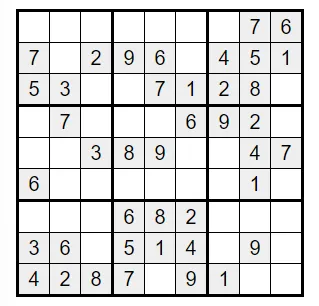
sudoku = [

[0, 0, 0, 0, 0, 0, 0, 7, 6],

[7, 0, 2, 9, 6, 0, 4, 5, 1],

[5, 3, 0, 0, 7, 1, 2, 8, 0],

[0, 7, 0, 0, 0, 6, 9, 2, 0],

[0, 0, 3, 8, 9, 0, 0, 4, 7],

[6, 0, 0, 0, 0, 0, 0, 1, 0],

[0, 0, 0, 6, 8, 2, 0, 0, 0],

[3, 6, 0, 5, 1, 4, 0, 9, 0],

[4, 2, 8, 7, 0, 9, 1, 0, 0]

]

solver = SudokuSolver(sudoku)

solution = solver.solve_sudoku()

if solution:

print("Sudoku solution:")

for row in solution:

print(row)

else:

print("No solution exists.")
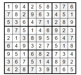
Solution:
Returns a 9×9 grid with final Sudoku values solved.
Real-Life Constraint Satisfaction Problems & Applications
Here are many different problems and real-life applications of Constraint Satisfaction Problems mentioned below:
- N-Queens Problem: As we discussed above, this problem refers to placing N queens on the NxN chessboard. These questions can have a very high number of total variable and domain combinations and hold more than one solution.
- Map Colouring: Colouring regions on a map, including many conditions like no adjacent colour match or vice-versa, or any other constraints.
- Sudoku Solver: CSPs can solve Sudoku faster than most of the algorithms present today. It can also solve sudoku for NxN size.
- Cryptarithmetic Puzzles: These puzzles have fill-in-the-blanks type questions, in which a single word can act as a whole unique digit. Their summation or subtraction will generate a new unknown word which is solved through CSPs.
- Magic Square: This is a fill-in-the-grid problem where you have to fit different digits into a cell such that the sums of the numbers in row, column and diagonal are equal.
- Word Search Puzzle: Classic word search puzzle to fill in different words from the given options or to match and complete the whole word, with constraints to be fit in rows, columns or diagonals.
- Zebra Puzzle: This problem also contains different constraints where you need to determine the arrangement of houses according to their inhabitants and other various attributes.
- Minesweeper Solver: To determine the location of mines in a minesweeper game based on different clues given in the grid.
- Latin Square: This game involves filling an NxN grid with different N symbols such that each symbol would appear exactly once in each row and column.
- Resource Allocation: CSPs can be highly essential in resource allocation as you need to allocate resources based upon certain constraints. Same with the task allocation where you divide tasks based on the resources’ types and other important constraints.
Conclusion
In conclusion, the Constraint Satisfaction Problem (CSP) forms a fundamental concept in artificial intelligence, where using only the frameworks and basic calculations, you can categorise, classify or find answers to constraining problems. It is important how you define constraint as it will impact the final solution and systematic exploration through various algorithms. You can implement the CSP algorithm yourself, which will make you aware of each and every function and data type used.
How are CSPs used in Artificial Intelligence?
What are the components of a CSP?
What are global constraints in CSPs?
What are soft constraints?
What is backtracking in CSPs?
How do heuristics improve CSP solving?
What is constraint propagation?
Updated on July 18, 2024