Join Our 4-Week Free Gen AI Course with select Programs.

Request a callback

or Chat with us on

Learning Hub

Articles

Bellman–Ford Algorithm – A Complete Guide

Basics of Python

5 Hrs. duration

9 Modules

1800+ Learners

Start Learning

The Bellman-ford algorithm is a well-known algorithm that solves the single-source shortest paths problem in a weighted directed graph. It is especially useful for cases when the graph has negative weight edges. Unlike Dijkstra’s algorithm, the Bellman-ford algorithm works even when edges in the graph are allowed to have negative weights and can also determine if the graph contains any negative weight cycles.

This guide will take you through a detailed exploration of the Bellman-Ford algorithm, starting with its foundations, workings, handling of negative weight cycles, pseudocode, variations from Dijkstra’s algorithm, code implementations in multiple languages, complexity analysis, and applications.

What is the Bellman-Ford Algorithm?

The Bellman-Ford algorithm determines the shortest paths from a single source vertex to all other vertices in a weighted graph. It does this by considering all edges in turn for each of the vertices. This paves the way for its notable feature of being able to handle graphs with negative weight edges. This distinguishes it from algorithms like Dijkstra’s, which work only for non-negative edge weights.

Bellman-Ford algorithm can be used on both weighted and unweighted graphs. In this algorithm, If there is a negative cycle in the graph, it is impossible to find the shortest path. The path’s cost will keep going down even while its length grows if we keep going around the negative cycle indefinitely. Bellman-Ford algorithm can therefore also identify negative cycles, which is a crucial aspect.

The Bellman-Ford algorithm is based on the principles of dynamic programming. It computes the shortest paths by iteratively relaxing every edge. Relaxation is updating the distance and predecessor values if a better path is found, in which further vertices can be connected only after relaxing that edge. The algorithm operates with iterations and in each of them goes through all edges, trying to “relax” them. This continues until no more updates are made for any vertex in the passes.

Characteristics:

Works with both directed and undirected graphs.
Detects negative weight cycles (a cycle whose total weight is negative)
Bellman-Ford is one of the well-known single-source shortest-path algorithms.
Does not guarantee the fastest runtime but guarantees correctness even for challenging cases.

How Does the Bellman-Ford Algorithm Work?

The foundation of the Bellman-Ford algorithm is dynamic programming. It relaxes each edge to determine the shortest pathways step-by-step. Comparing and updating the shortest path estimate if a shorter path is discovered is the process known as relaxation. The method checks every edge and attempts to improve the shortest path estimate throughout each iteration. Here are the step-by-step workings of the Bellman-Ford algorithm:

Step 1: Initialisation

Set the distance from the source vertex to itself as 0, and to all other vertices as infinity.

for each vertex v in Graph:

if v == source:

distance[v] = 0

else:

distance[v] = ∞

Step 2: Relaxing the edges

For each edge, if the distance to the destination vertex can be shortened by going through the source vertex, update the destination’s distance.

for i from 1 to |V|-1:

for each edge (u, v) in Graph:

if distance[u] + weight(u, v) < distance[v]:

distance[v] = distance[u] + weight(u, v)

Step 3: Check for Negative Cycles

Repeat the relaxation step V−1 times for each edge in the graph, where V is the number of vertices. Complete one more relaxing step following V−1 iterations. A negative weight cycle exists if any distance is updated.

for each edge (u, v) in Graph:

if distance[u] + weight(u, v) < distance[v]:

print “Graph contains a negative-weight cycle”

return

Step 4: Shortest paths

The final step is to return the shortest path. If there are no negative cycles in the graph, the shortest path from the source node to all other nodes of the graph is returned.

return distance

How does Bellman-Ford Algorithm Handle Negative Weight Edges & Cycles?

Bellman-Ford algorithm has a key strength in handling the negative weight edges and cycles in the graph. Let’s see how it handles both:

Negative Weight Edges

Negative weight edges can be present in graphs if the existence of certain transitions or paths would mean a decrease in cost (or distance) from what has already been computed. The Bellman-Ford correctly computes the shortest path even when such edges exist by allowing for multiple relaxations of edges.

Negative Weight Cycles

A negative weight cycle is when a cycle in the graph has a total sum of weights that is negative. In this situation, no shortest path will exist because the algorithm could keep reducing the path cost by travelling around the cycle indefinitely.

If after V−1 relaxations no edges can be relaxed and some can still be relaxed, then a negative weight cycle is present.
The Bellman-Ford algorithm discovers this and indicates the presence of negative weight cycles by returning a special value to the user so that it should be thought of as a way of warning that, in such cases, the shortest path cannot be computed in a well-defined way.

Pseudocode of Bellman-Ford Algorithm

Here is the pseudocode for the bellman-ford algorithm:

function BellmanFord(Graph, source):

// Step 1: Initialise distances

for each vertex v in Graph:

if v == source:

distance[v] = 0

else:

distance[v] = ∞

// Step 2: Relax edges |V|-1 times

for i from 1 to |V|-1:

for each edge (u, v) in Graph:

if distance[u] + weight(u, v) < distance[v]:

distance[v] = distance[u] + weight(u, v)

// Step 3: Check for negative-weight cycles

for each edge (u, v) in Graph:

if distance[u] + weight(u, v) < distance[v]:

print “Graph contains a negative-weight cycle”

return

// Shortest Path

return distance

Explanation:

Initialisation: The distance to the source is set to 0, and all other distances are initialised to infinity.
Relaxation: For each edge, check if a shorter path can be found. If so, update the shortest path estimate.
Negative Cycle Check: After relaxing the edges V−1 times, check once more for negative-weight cycles.

Bellman-Ford Algorithm Example

For this example, consider a graph with 5 vertices (A, B, C, D, E) with the following edges having weights:

A -> B (weight 2)

A -> C (weight 3)

B -> D (weight 1)

C -> D (weight 6)

B -> E (weight 4)

D -> E (weight -1)

Bellman-Ford Algorithm Example

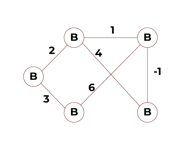
From the given graph weights, we will run the Bellman-Ford algorithm to determine the shortest path from vertex (node) A to all other vertices (nodes).

Step 1: Initialisation

The first step is to initialise all other vertices’ distances to infinity (∞) and the distance to the source vertex A to 0. We also keep track of the parent of each vertex (used to reconstruct paths).

Vertex	Distance from A	Parent
A	0	–
B	∞	–
C	∞	–
D	∞	–
E	∞	–

Step 2: Relaxing the edges

In this step, we try to discover the shortest path to each vertex by relaxing each edge in the graph. V is the number of vertices, and we repeat this method V−1 times. This makes sure we take into consideration all potential shortest paths.

Iteration 1:

A -> B (distance(B) = min(∞, 0 + 2) = 2
A -> C (distance(C) = min(∞, 0 + 3) = 3
B -> D (distance(D) = min(∞, 2 + 1) = 3
C -> D (distance(D) = min(3, 3 + 6) = 3 (no change)
B -> E (distance(E) = min(∞, 2 + 4) = 6
D -> E (distance(E) = min(6, 3 + (-1)) = 2

Vertex	Distance from A	Parent
A	0	–
B	2	A
C	3	A
D	3	B
E	2	D

Iteration 2:

A -> B (distance(B) = 2), no change
A -> C (distance(C) = 3), no change
B -> D (distance(D) = 2), no change
C -> D (distance(D) = 3), no change
B -> E (distance(E) = 2), no change
D -> E (distance(E) = 2), no change

Iteration 3: All distances are unchanged after the third iteration of the algorithm.

Iteration 4: All distances are unchanged after the fourth iteration of the algorithm.

Step 3: Checking negative cycles

We now check the graph to see if there are any negative weight cycles following the V−1 iterations. To do this, try to relax each edge only once more. If any distance can be reduced further, it means that the graph contains a negative weight cycle.

In our example,

A -> B (distance(B) = 2), no change
A -> C (distance(C) = 3), no change
B -> D (distance(D) = 2), no change
C -> D (distance(D) = 3), no change
B -> E (distance(E) = 2), no change
D -> E (distance(E) = 2), no change

Since no distances can be further reduced, we confirm that the graph does not contain any negative weight cycles, and can now move to determine shortest paths.

Step 4: Shortest paths

We can now output the shortest paths from vertex A to every other vertex after the relaxation is finished and it is verified that there are no negative weight cycles.

Vertex	Distance from A	Parent
A	0	A
B	2	A -> B
C	3	A -> C
D	3	A -> B -> D
E	2	A -> B -> D -> E

From the above table, we can finally output our shortest paths as:

The shortest path from A to B is A -> B with a distance of 2.
The shortest path from A to C is A -> C with a distance of 3.
The shortest path from A to D is A -> B -> D with a distance of 3.
The shortest path from A to E is A -> B -> D -> E with a distance of 2.

Difference between Dijkstra’s and Bellman Ford’s Algorithm

Several differences differentiate Dijkstra’s algorithm from the Bellman-Ford algorithm. Below are some of the common and main differences between them:

Criteria	Dijkstra’s Algorithm	Bellman Ford’s Algorithm
Algorithm Type	The Dijkstra algorithm is implemented using the Greedy approach.	Bellman-Ford algorithm is implemented using Dynamic Programming.
Edge Weights	This algorithm can only non-negative weights.	This can handle both positive and negative weights.
Complexity	O (V^2) or O (E + V log V)	O (V E)
Negative Weight Cycles	Cannot handle negative weight cycles.	Detects negative weight cycles
Initial Distance Values	All distances are set to infinity, except the source.	All distances are set to infinity, except the source.
Edge Relaxation	It relaxes edges based on the unprocessed closest vertex.	Updates the shortest path by relaxing each edge in each iteration.
Graph Used	It can work on both directed as well as undirected graphs.	It can also work on both directed as well as undirected graphs.
Optimal for Real-Time Systems	Yes, it is optimal for real-time due to its efficiency and speed in non-negative graphs.	It is not optimal for real-time systems as it has a higher time complexity.
Distributed System	It is not easier to implement this algorithm in a distributed way.	It is easier to implement this algorithm in a distributed way.
Use Case	Faster for non-negative edge graphs.	Suitable for graphs with negative weights.

Code Examples

We will now understand the workings of the Bellman-Ford algorithm through code examples in different languages.

Bellman-Ford Algorithm Implementation in C

Code:

#include <stdio.h>

#include <limits.h>

#define INF INT_MAX

// Create an Edge Structure

struct Edge {

int src;

int d;

int weight;

};

// Function to run Bellman-Ford algorithm

void BellmanFord(int vertices, int edges, struct Edge edge[], int source) {

int distance[vertices];

// Step 1: Initialise distances from the source to all other vertices as INFINITY

for (int i = 0; i < vertices; i++) {

distance[i] = INF;

}

distance[source] = 0;

 

// Step 2: Relax all edges V-1 times

for (int i = 1; i <= vertices - 1; i++) {

for (int j = 0; j < edges; j++) {

int u = edge[j].src;

int v = edge[j].d;

int weight = edge[j].weight;

if (distance[u] != INF && distance[u] + weight < distance[v]) {

distance[v] = distance[u] + weight;

}

}

}

 

// Step 3: Check for negative-weight cycles

for (int i = 0; i < edges; i++) {

int u = edge[i].src;

int v = edge[i].d;

int weight = edge[i].weight;

if (distance[u] != INF && distance[u] + weight < distance[v]) {

printf("Graph contains negative-weight cyclen");

return;

}

}

 

// Step 4: Print the distances

printf("Vertex Distance from Sourcen");

for (int i = 0; i < vertices; i++) {

printf("%d tt %dn", i, distance[i]);

}

}

 

int main() {

int vertices = 5; // Number of vertices

int edges = 6;    // Number of edges

 

struct Edge edge[edges];

 

// Defining the graph with edges

edge[0].src = 0; edge[0].d = 1; edge[0].weight = 2;

edge[1].src = 0; edge[1].d = 2; edge[1].weight = 3;

edge[2].src = 1; edge[2].d = 3; edge[2].weight = 1;

edge[3].src = 2; edge[3].d = 3; edge[3].weight = 6;

edge[4].src = 1; edge[4].d = 4; edge[4].weight = 4;

edge[5].src = 3; edge[5].d = 4; edge[5].weight = -1;

 

int source = 0; // Source vertex

BellmanFord(vertices, edges, edge, source);

 

return 0;

}

Output:

Vertex Distance from Source

0 0

1 2

2 3

3 3

4 2

Bellman-Ford Algorithm Implementation in C++

Code:

#include <iostream>

#include <vector>

#include <climits>

using namespace std;

// Create an Edge Structure

struct Edge {

int src, dest, weight;

};

// Bellman-Ford algorithm

void BellmanFord(int vertices, int edges, vector<Edge>& edgeList, int source) {

vector<int> distance(vertices, INT_MAX);

distance[source] = 0;

// Relax all edges V-1 times

for (int i = 1; i <= vertices - 1; i++) {

for (int j = 0; j < edges; j++) {

int u = edgeList[j].src;

int v = edgeList[j].dest;

int weight = edgeList[j].weight;

if (distance[u] != INT_MAX && distance[u] + weight < distance[v]) {

distance[v] = distance[u] + weight;

}

}

}

// Check for negative-weight cycles

for (int i = 0; i < edges; i++) {

int u = edgeList[i].src;

int v = edgeList[i].dest;

int weight = edgeList[i].weight;

if (distance[u] != INT_MAX && distance[u] + weight < distance[v]) {

cout << "Graph contains negative-weight cycle" << endl;

return;

}

}

// Print the distances

cout << "Vertex Distance from Source" << endl;

for (int i = 0; i < vertices; i++) {

cout << i << "tt" << distance[i] << endl;

}

}

int main() {

int vertices = 5; // Number of vertices

int edges = 6;    // Number of edges

vector<Edge> edgeList(edges);

// Defining the graph with edges

edgeList[0] = {0, 1, 2};

edgeList[1] = {0, 2, 3};

edgeList[2] = {1, 3, 1};

edgeList[3] = {2, 3, 6};

edgeList[4] = {1, 4, 4};

edgeList[5] = {3, 4, -1};

int source = 0; // Source vertex

BellmanFord(vertices, edges, edgeList, source);

 

return 0;

}

Output:

Vertex Distance from Source

0 0

1 2

2 3

3 3

4 2

Bellman-Ford Algorithm Implementation in Java

Code:

import java.util.Arrays;

class BF {

// Edge class to represent each edge

static class Edge {

int src, d, weight;

Edge(int src, int d, int weight) {

this.src = src;

this.d = d;

this.weight = weight;

}

}

 

// Bellman-Ford algorithm

void BellmanFordAlgorithm(int vertices, Edge[] edges, int source) {

int[] distance = new int[vertices];

Arrays.fill(distance, Integer.MAX_VALUE);

distance[source] = 0;

 

// Relax all edges V-1 times

for (int i = 1; i <= vertices - 1; i++) {

for (Edge edge : edges) {

if (distance[edge.src] != Integer.MAX_VALUE &&

distance[edge.src] + edge.weight < distance[edge.d]) {

distance[edge.d] = distance[edge.src] + edge.weight;

}

}

}

 

// Check for negative-weight cycles

for (Edge edge : edges) {

if (distance[edge.src] != Integer.MAX_VALUE &&

distance[edge.src] + edge.weight < distance[edge.d]) {

System.out.println("Graph contains negative-weight cycle");

return;

}

}

 

// Print the distances

System.out.println("Vertex Distance from Source");

for (int i = 0; i < vertices; i++) {

System.out.println(i + "tt" + distance[i]);

}

}

 

public static void main(String[] args) {

int vertices = 5; // Number of vertices

int edgeCnt = 6; // Number of edges

 

Edge[] edges = new Edge[edgeCnt];

 

// Defining the graph with edges

edges[0] = new Edge(0, 1, 2);

edges[1] = new Edge(0, 2, 3);

edges[2] = new Edge(1, 3, 1);

edges[3] = new Edge(2, 3, 6);

edges[4] = new Edge(1, 4, 4);

edges[5] = new Edge(3, 4, -1);

 

BF bf = new BF();

bf.BellmanFordAlgorithm(vertices, edges, 0);

}

}

Output:

Vertex Distance from Source

Explanation:

In all three example codes, firstly all vertices in the distance array are initialised to infinity (or the maximum value), and the source vertex is set to 0.
We then update the distances based on edge weights by iterating over all edges V−1 times, where V is the number of vertices.
A final check is performed by trying to relax all edges one more time following V−1 iterations. If there is still a reduction in distance, there is a negative-weight cycle present.
Finally, the shortest path between the source vertex and each of the remaining vertices is printed.

Internship Assurance

DevOps & Cloud Engineering

Explore

Complexity Analysis of Bellman-Ford Algorithm

Time Complexity

The Bellman-Ford algorithm has a time complexity of O(V * E). Let’s see how and when:

Best Case Time Complexity:

In the best case O(V * E), the Bellman-Ford will still run as it has to go through the relaxation step for all edges, even if no updates are required after the first few iterations. It does not stop prematurely like Dijkstra’s algorithm when all shortest paths have been found; therefore, the algorithm goes on V−1 iterations even if the solution has stabilised earlier.

For example, in case the input graph contains no negative weight edges and after one relaxation all distances are computed, Bellman-Ford would still go ahead with the remaining V−2 iterations.

Worst Case Time Complexity:

The worst case for the Bellman-Ford algorithm is when the graph has V large number of edges E relative to vertices (such as in a dense graph), the graph contains negative weight edges and a full set of V−1 relaxations must be done, the graph may have a negative weight cycle but still completes all relaxation steps before detecting that cycle. Therefore, the time complexity in the worst case will remain O(V * E).

Space Complexity

The Bellman-Ford algorithm has an O(V + E) space complexity.

Distance Array (O(V)):

To store the shortest path estimates from the source vertex to each other vertex, the method keeps track of a distance array. O(V) space is required for this array, where V is the number of vertices.

List of Edges (O(E)):

Typically, the graph is shown as an edge list, with each edge connecting two vertices assigned a weight. O(E) space is needed in the edge list to hold all of the edges.

As a result, O(V + E) is the total space complexity, taking into consideration the edge list and distance array storage.

Applications of Bellman-Ford Algorithm

Various domains such as computer networks, distributed systems, optimisation problems, etc., make extensive use of the Bellman-Ford algorithm. Here are various applications of the Bellman-Ford algorithm:

Computer Networks: The algorithm is commonly used in distance vector routing protocols of computer networks such as the Routing Information Protocol (RIP) to calculate the shortest mesh network based on weighted edges.
Currency Arbitrage: Negative cycles are regarded as successive trades that can be completed for a profit and can therefore be classified using the Bellman-Ford algorithm for negative cycle detection.
Distributed Systems: This algorithm could be useful for solving the problem in a distributed computer system where processes work together but need to communicate with each other and explore the best paths.
Pathfinding in Games: It can be applied in games for spatial pathfinding across different game objects or entities with fouls and penalty points incurred for movement through specific paths toward the goals.
Arbitrage Detection: In undertaking loss minimisation in a network of capital flow graphs, arbitrage detection involves locating negative weight cycles.
Detecting Negative Weight Cycles: The algorithm detects negative weight cycles in a graph, which may be a sign of problems such as financial arbitrage or unsustainable activities.
Operations Research: As far as network design optimisation or logistics practice is concerned the Bellman-Ford approaches aid in network routing for the minimum path problems where the distance cost or delay is the most in certain paths used.

Conclusion

The Bellman-Ford algorithm is an important part of graph theory, especially in the case of negative edge-weighted graphs. It guarantees the validity of the shortest path in these cases and even finds negative weight cycles. However, it will cease being the best algorithm for large-scale problems, but only positive weights will have Dijkstra’s ability’s scope. This is particularly useful in a multiplicity of fields.

Be it in computer networks, financial markets, games, or any others, Bellman-Ford is an algorithm that represents the basics of dynamic programming applicable in solving non-trivial graph problems. To sum up, the best way to quickly explain the key algorithm for solving negative weights or negative cycles is the Bellman-Ford algorithm.

Deploying Applications Over the Cloud Using Jenkins

Prashant Kumar Dey

Associate Program Director - Hero Vired

Ex BMW | Google

19 October, 12:00 PM (IST)

Limited Seats Left

Book a Free Live Class

Programs tailored for your success

Popular

Management

Data Science

Finance

Technology

Future Tech

3 ASSURED INTERVIEWS

Accelerator Program in

Business Analytics and Data Science

With

Part-time · 10 months

Apply by : 19 October, 2024

Financial Analysis, Valuation, & Risk Management

3 ASSURED INTERVIEWS

Certificate Program in

Financial Analysis, Valuation, & Risk Management

With

Part-time · 7 months

Apply by : 19 October, 2024

INTERNSHIP ASSURANCE

Certificate Program in

DevOps & Cloud Engineering

With

Part-time · 7.5 months

Apply by : 19 October, 2024

Upskill with expert articles

View all

Hero Vired is a leading LearnTech company dedicated to offering cutting-edge programs in collaboration with top-tier global institutions. As part of the esteemed Hero Group, we are committed to revolutionizing the skill development landscape in India. Our programs, delivered by industry experts, are designed to empower professionals and students with the skills they need to thrive in today’s competitive job market.

Data Science

Accelerator Program in Business Analytics & Data Science

Integrated Program in Data Science, AI and ML

Accelerator Program in AI and Machine Learning

Advanced Certification Program in Data Science & Analytics

Technology

Certificate Program in Full Stack Development with Specialization for Web and Mobile

Certificate Program in DevOps and Cloud Engineering

Certificate Program in Application Development

Certificate Program in Cybersecurity Essentials & Risk Assessment

Finance

Integrated Program in Finance and Financial Technologies