The first step in Merge Sort is to divide the array. We split the array into two halves until each sub-array contains a single element. This step is straightforward but crucial for the divide and conquer strategy.
Consider the array: [38, 27, 43, 3, 9, 82, 10].
At this point, each sub-array has one element.
Next, we sort each sub-array. Since each sub-array has only one element, they are already sorted. The conquer phase focuses on preparing these small arrays for the merging process.
The final step is to merge the sorted sub-arrays back together. This step involves comparing elements from each sub-array and combining them into a single sorted array.
def merge_sort(arr):
if len(arr) > 1:
mid = len(arr) // 2
left_half = arr[:mid]
right_half = arr[mid:]
merge_sort(left_half)
merge_sort(right_half)
i = j = k = 0
while i < len(left_half) and j < len(right_half):
if left_half[i] < right_half[j]:
arr[k] = left_half[i]
i += 1
else:
arr[k] = right_half[j]
j += 1
k += 1
while i < len(left_half):
arr[k] = left_half[i]
i += 1
k += 1
while j < len(right_half):
arr[k] = right_half[j]
j += 1
k += 1
arr = [38, 27, 43, 3, 9, 82, 10]
merge_sort(arr)
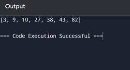
print(arr)
Output
The output of this code will be:

POSTGRADUATE PROGRAM IN
Multi Cloud Architecture & DevOps
Master cloud architecture, DevOps practices, and automation to build scalable, resilient systems.
Detailed Breakdown of Merge Sort’s Time Complexity
Best Case Time Complexity
In ideal circumstances, the array is already arranged. Merge Sort keeps working even if it seems like we won’t need to sort it again. Since the elements are already sorted, fewer comparisons are needed when the array is divided and merged as usual.
Let’s consider an already sorted array: [1, 2, 3, 4, 5, 6, 7].
- Divide Phase:
- Conquer Phase:
- [1, 2, 3] becomes [1], [2], [3]
- [4, 5, 6, 7] becomes [4], [5], [6], [7]
- Combine Phase:
- [1] and [2] merge to [1, 2], then [1, 2] and [3] merge to [1, 2, 3]
- [4] and [5] merge to [4, 5], then [4, 5] and [6] merge to [4, 5, 6], then [4, 5, 6] and [7] merge to [4, 5, 6, 7]
- Finally, [1, 2, 3] and [4, 5, 6, 7] merge to [1, 2, 3, 4, 5, 6, 7]
Because the elements are already ordered, fewer comparisons are made during the merging process in this case. However, due to the splitting and merging processes, the time complexity remains O(n log n).
Average Case Time Complexity
The most typical case occurs when the components are jumbled together but not completely out of order. Here, the comparisons and swaps will be distributed more evenly throughout the operation.
Consider an array: [10, 5, 2, 8, 7, 3, 6].
- Divide Phase:
- Conquer Phase:
- [10, 5, 2] becomes [10], [5], [2]
- [8, 7, 3, 6] becomes [8], [7], [3], [6]
- Combine Phase:
- [10] and [5] merge to [5, 10], then [5, 10] and [2] merge to [2, 5, 10]
- [8] and [7] merge to [7, 8], then [7, 8] and [3] merge to [3, 7, 8], then [3, 7, 8] and [6] merge to [3, 6, 7, 8]
- Finally, [2, 5, 10] and [3, 6, 7, 8] merge to [2, 3, 5, 6, 7, 8, 10]
The time complexity is still O(n log n) in this typical situation. Splitting and merging are done in each phase, along with an equal number of swaps and comparisons.
Worst Case Time Complexity
When the array is sorted in reverse order, the worst-case situation occurs. In this scenario, the quantity of comparisons and swaps required during the merging processes is maximised.
Consider an array: [7, 6, 5, 4, 3, 2, 1].
- Divide Phase:
- Conquer Phase:
- [7, 6, 5] becomes [7], [6], [5]
- [4, 3, 2, 1] becomes [4], [3], [2], [1]
- Combine Phase:
- [7] and [6] merge to [6, 7], then [6, 7] and [5] merge to [5, 6, 7]
- [4] and [3] merge to [3, 4], then [3, 4] and [2] merge to [2, 3, 4], then [2, 3, 4] and [1] merge to [1, 2, 3, 4]
- Finally, [5, 6, 7] and [1, 2, 3, 4] merge to [1, 2, 3, 4, 5, 6, 7]
Even in this worst case, the time complexity remains O(n log n). The key difference lies in the number of comparisons and swaps required to merge the sub-arrays.
In-depth Analysis of Merge Sort’s Space Complexity
General Space Complexity
Merge Sort is known for its efficient time complexity, but it also requires additional memory. Its space complexity is O(n). This means that, in addition to the input array, we need extra space equal to its size.
Why does Merge Sort need extra space? When we merge two sorted halves, we use an auxiliary array to hold the merged result before copying it back to the original array. This auxiliary array is crucial for the merge process. Let’s look at an example to understand this better.
Example of Space Usage
Consider an array: [38, 27, 43, 3, 9, 82, 10].
- Divide Phase:
- [38, 27, 43]
- [3, 9, 82, 10]
- Conquer Phase:
- [38, 27, 43] becomes [38], [27], [43]
- [3, 9, 82, 10] becomes [3], [9], [82], [10]
- Combine Phase:
- [38] and [27] merge to [27, 38], then [27, 38] and [43] merge to [27, 38, 43]
- [3] and [9] merge to [3, 9], then [3, 9] and [82] merge to [3, 9, 82], then [3, 9, 82] and [10] merge to [3, 9, 10, 82]
- Finally, [27, 38, 43] and [3, 9, 10, 82] merge to [3, 9, 10, 27, 38, 43, 82]
Throughout the merge process, we use extra space equivalent to the size of the array.

82.9%
of professionals don't believe their degree can help them get ahead at work.
Using Linked Lists to Optimise Space
Can we optimise space complexity? Yes, using linked lists can help. With linked lists, we can merge in place, avoiding the need for a large auxiliary array. Instead, we only need space for the recursion stack. This reduces the space complexity to O(log n).
Using the same array but represented as a linked list, the merge process works directly on the list nodes, reducing space overhead. This approach is beneficial in memory-constrained environments. However, implementing Merge Sort with linked lists can be more complex.
Recursion and Stack Frames
Merge Sort is a recursive algorithm. Each recursive call adds a frame to the stack, contributing to space complexity. The maximum depth of recursion is log n, so the stack space needed is O(log n). While this is less than the O(n) for the auxiliary array, it still impacts the overall space complexity.
Practical Considerations
In practical applications, the space complexity of Merge Sort affects performance, especially with large datasets. The extra space requirement can be a drawback compared to in-place sorting algorithms like Quick Sort. However, the stability and predictable performance of Merge Sort often outweigh these considerations.
Practical Implications of Parallelising Merge Sort
Parallelising Merge Sort can potentially speed up the sorting process. By dividing the work among multiple processors, we can sort large datasets more efficiently. But what are the real benefits and challenges of this approach?
Benefits of Parallelising Merge Sort
Parallelising Merge Sort can significantly reduce sorting time. Each processor handles a part of the array independently. After sorting their parts, processors then merge the results. This parallel processing can be faster, especially for large datasets.
Challenges of Parallelising Merge Sort
While the theory sounds promising, there are practical challenges. Synchronisation between processors can introduce overhead. Managing multiple processors also adds complexity. Moreover, not all systems support efficient parallel processing.
Example of Parallel Merge Sort
Let’s look at a simple example using Python:
import multiprocessing
def merge_sort_parallel(arr, pool):
if len(arr) > 1:
mid = len(arr) // 2
left_half = arr[:mid]
right_half = arr[mid:]
pool.apply_async(merge_sort_parallel, (left_half, pool))
pool.apply_async(merge_sort_parallel, (right_half, pool))
left_half = merge_sort_parallel(left_half, pool)
right_half = merge_sort_parallel(right_half, pool)
i = j = k = 0
while i < len(left_half) and j < len(right_half):
if left_half[i] < right_half[j]:
arr[k] = left_half[i]
i += 1
else:
arr[k] = right_half[j]
j += 1
k += 1
while i < len(left_half):
arr[k] = left_half[i]
i += 1
k += 1
while j < len(right_half):
arr[k] = right_half[j]
j += 1
k += 1
return arr
if __name__ == “__main__”:
arr = [38, 27, 43, 3, 9, 82, 10]
pool = multiprocessing.Pool(processes=4)
sorted_arr = merge_sort_parallel(arr, pool)
pool.close()
pool.join()
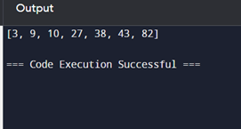
print(sorted_arr)
Output
The output will be:
Practical Considerations
Before deciding to parallelise Merge Sort, consider the hardware and the size of the dataset. For small arrays, the overhead may not justify the speedup. For larger datasets on suitable hardware, the benefits can be substantial.
Comparison of Merge Sort with Other Sorting Algorithms
Quick Sort vs. Merge Sort
Both Quick Sort and Merge Sort are very efficient data sorting algorithms despite the fact that they have different capabilities. Because the overhead is kept to a minimum, Quick Sort is relatively faster. But, one should also keep in mind that it has a worst-case time complexity of O(n²) while Merge Sort has O(n log n). One more difference that needs to be highlighted is that while Merge Sort is an example of a stable algorithm, meaning that it keeps the order of equal elements intact, Quick Sort is an example of an unstable sorting algorithm.
Insertion Sort vs. Merge Sort
The insertion sort algorithm is best suited for small numbers of elements and partially sorted elements. In the best case, it has a time complexity of O(n). Thus, Merge Sort is preferable for larger data collections due to its O(n log n) time complexity. Like many sorting algorithms, Insertion Sort is often used in conjunction with other algorithms for small subarrays.
Bubble Sort vs. Merge Sort
Bubble Sort is a data sorting algorithm which is very easy to understand and implement, but because of its time complexity O(n²), efficiency is very low. This is the reason why it can’t be used for larger data sets. Therefore, for large arrays, Merge Sort, with its time complexity of O(n log n), is more efficient. Bubble sort is useful for educational settings and small arrays since its technique is very simple to implement.
Comparison Table
| Algorithm |
Time Complexity (Best) |
Time Complexity (Average) |
Time Complexity (Worst) |
Space Complexity |
Stability |
| Merge Sort |
O(n log n) |
O(n log n) |
O(n log n) |
O(n) |
Stable |
| Quick Sort |
O(n log n) |
O(n log n) |
O(n²) |
O(log n) |
Unstable |
| Bubble Sort |
O(n) |
O(n²) |
O(n²) |
O(1) |
Stable |
| Insertion Sort |
O(n) |
O(n²) |
O(n²) |
O(1) |
Stable |
Conclusion
Merge Sort can be recognised as one of the most efficient and stable sorting algorithms. We went through the details of how the divide and conquer strategy can sort arrays, hence making the step-by-step process easy to understand. We discussed how it has ‘O(n log n)’ time complexity, which is appropriate for different circumstances, including the worst-case. We looked at its space complexity, noting that the auxiliary array has an O(n) requirement and discussing how linked lists may assist in improving it.
We also discussed the feasibility of parallelising Merge Sort and looked at the opportunities and possible issues in doing so. Comparing it with other algorithms like Quick Sort, Bubble Sort, and Insertion Sort helped us understand some of the outstanding features of Merge Sort, such as its stability and relative speed. Knowing these aspects, we can apply Merge Sort in sorting different types of problems with confidence and, therefore, add it to our list of algorithms.
